More on data visualization
More details on data visualization. Know-how and -why of aesthetics. Basic themes and extensions. Guides: axes, labels, scales, breaks, and legends. Statistical transformations. Text and annotations.
1 Prerequisites
- We examine some aspects of
ggplot2in more detail.
- We will use the
eu_ictandictdata frames in our visualizations.
2 Programming digression: argument passing
- In the visualization overview topic, we have followed the convention of explicitly specifying the arguments of functions.
- This is not a necessity.
2.1 Argument order and named arguments
- There are three ways to pass arguments to functions in
R.
- By exact matching.
- By partial matching.
- By position.
2.2 Exact matching
- By exact matching.
- We specify the argument name and the value.
- The names of the arguments are documented in the help files of the functions.
- Documentation is available with
?function_name.
Exact matching
- By exact matching.
2.3 Partial matching
- By partial matching.
- We specify partially the argument name and the value.
- We can provide the minimum number of initial characters (or more) that uniquely identify the argument.
Partial matching
- By partial matching.


2.4 Positional arguments
- By position
- We specify only values.
- Arguments are matched by their position in the function signature.
Positional arguments
- By position

Positional arguments
- The same applies to the
aes()function.

2.5 Why so many ways?
- Each approach has pros and cons.
Why so many ways?
- Exact matching is quite verbose.
- But it is self-documenting and less error-prone.
- It is a good practice to use it when readability is important. For example:
- In scripts that are shared with others that are not familiar with the used functions.
- When calling functions that you do not use frequently, and you might need to revisit the code after a long time.
Why so many ways?
- Positional matching is concise.
It is a good practice to use it for commonly used functions where the risk of confusion is low. E.g.,
instead of
Using it in
R’s command line for experimentation can be easier.But it can make reading code less self-contained.
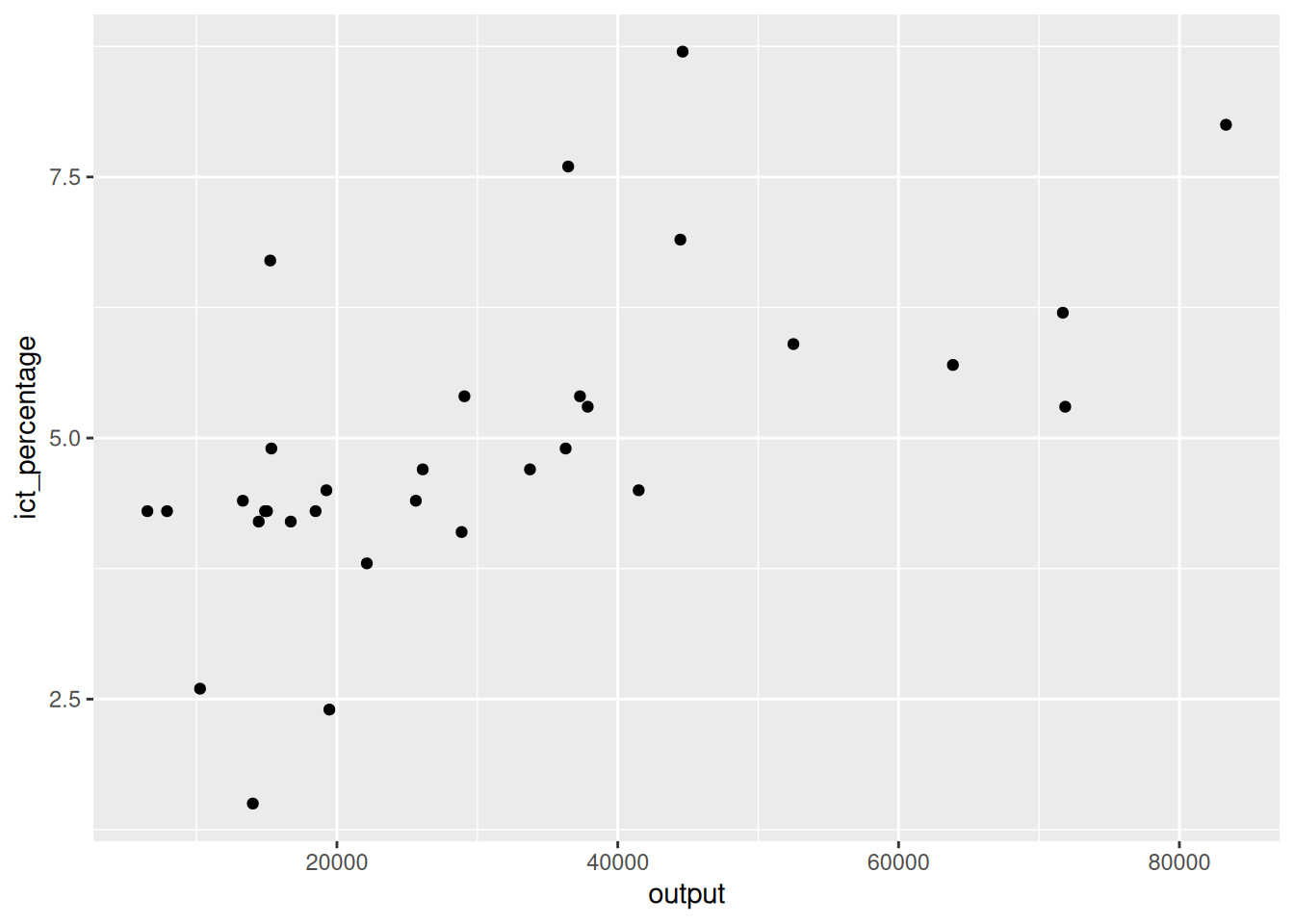
3 Aesthetics mappings
- In the visualization overview topic, we used
aesto add or modify the appearance of plot elements.
3.1 Defining aesthetics
- Aesthetics can be defined at various levels when creating a plot.

Defining aesthetics
- Aesthetics can be defined at various levels when creating a plot.
Defining aesthetics
- Aesthetics can be defined at various levels when creating a plot.

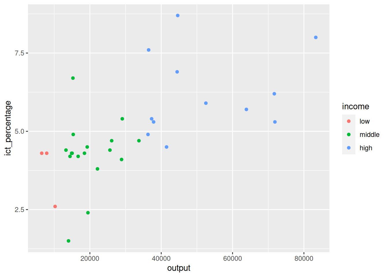
3.2 Defining aesthetics: how
- How does this work?
3.3 Defining aesthetics: why
- Why does it work in this way?
- We can specify the aesthetics of certain layers with attributes that we do not want to apply globally.
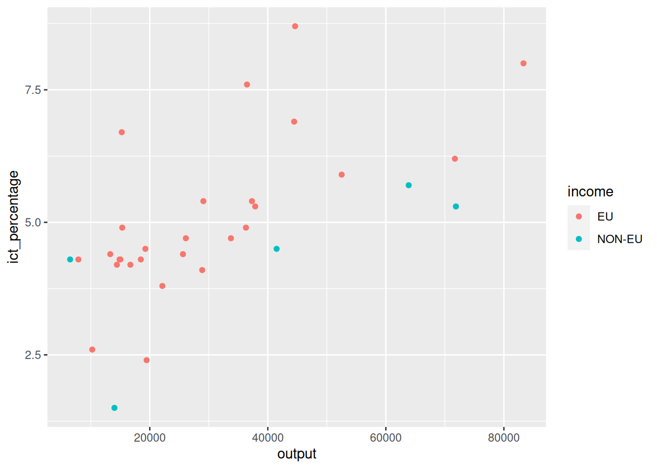
3.4 Defining aesthetics: why
- Why does it work in this way?

Defining aesthetics
- Why does it work in this way?

4 Theming
- Aesthetics modify the appearance of the plot’s data elements.
- How can we modify the appearance of the plot’s non-data elements (e.g., axes, background, grid)?
- The
ggplot2package provides a set of eight basic themes.
4.1 Basic themes
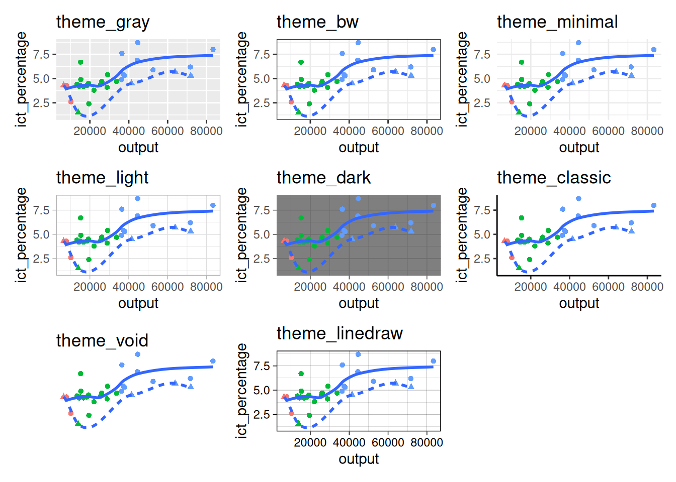
Basic themes
Basic themes
- We can apply themes to the plot by adding them with the
+operator.
Basic themes
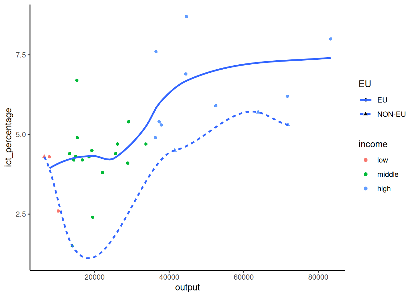
- Themes only affect the non-data elements of the plot.
Basic themes
- Themes only affect the non-data elements of the plot.
Basic themes
- Themes only affect the non-data elements of the plot.
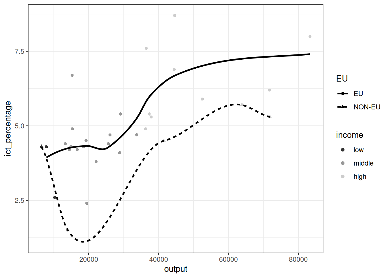
- Here, we have combined the
theme_bw()withscale_color_grey()to modify the appearance of the data elements. - In addition, we have explicitly specified the color of the
geom_smooth()object to be black.
4.2 Additional themes
- If the basic themes do not meet the stylistic requirements that you want or being asked to follow, taking a look at the
ggthemespackage is a good idea.
Additional themes
- The
ggthemespackage provides additional themes that might match the desired style.

5 Guides
- Guides are reference lines, grids, or markers assisting in interpreting the geometric object of the visualization.
- Axes and legends are the two guides that are most commonly modified in a visualization to facilitate communication.
5.1 Axes
- Axes are the typically horizontal and vertical lines that specify the coordinate system of the plot area.
- Axes have breaks (ticks) and labels.
- Breaks are the marked points of an axis.
- Labels are the text accompanying the breaks and provide interpretation context for the axis.
5.2 Labels
- We have seen in the visualization overview topic how to modify the axes labels of a visualization via the
labs()function.
Labels

Labels
Labels
- How can we modify the breaks of an axis?
- How can we modify the labels of these breaks?
Labels
- Not very intuitively, the breaks and labels of an axis are not modified through
labs().
- This is because
ggplot2does some heavy lifting for us when drawing the axes of a plot. - Recall that we have used the same calling interface for creating plots with continuous and discrete axes variables (e.g.,
geom_pointandgeom_bar).
5.3 Scales
- In the background,
ggplot2automatically adjusts the axes based on the type of the variable we provide.
- It does so by using the
scale_*()family of functions. - Scales are instructions controlling how certain aesthetic mappings are translated into visual properties.
- For example, a continuous scale maps the values of an aesthetic to a continuous axis range.
Scales
- In
ggplot2, continuous variables ingeom_point()objects are automatically assigned to a continuous scalescale_x_continuous().
- Discrete variables in
geom_bar()objects are automatically assigned to a discrete scalescale_color_discrete(). - We can modify the default behavior and the appearance of axes by explicitly calling the
scale_*()functions.
5.4 Breaks
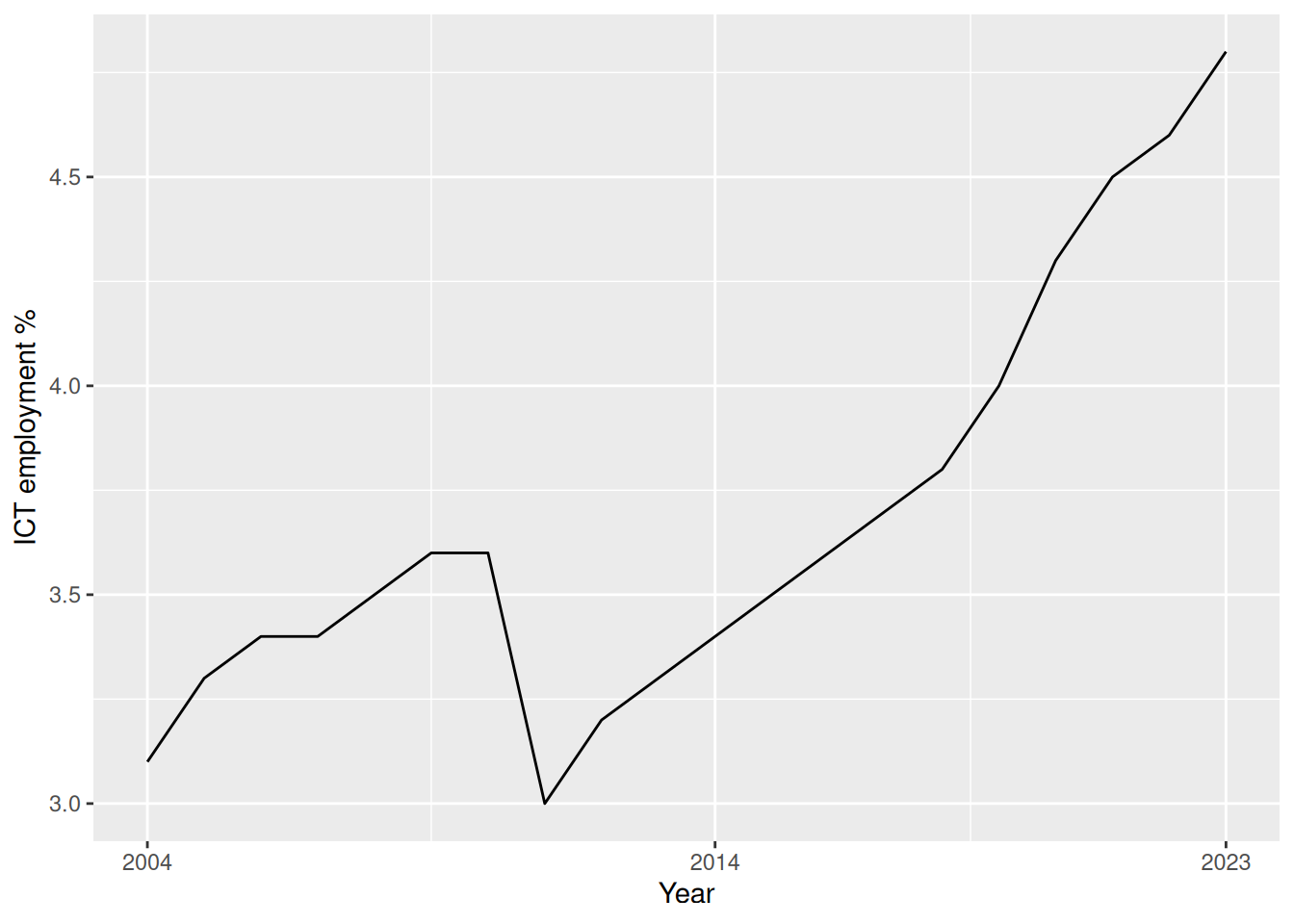
- We can pass directly the breaks we want to have on a continuous axis using the
breaksargument.
- For instance, if we want to have all the years as breaks, we can pass the
yearcolumn of theictdata frame.
Breaks
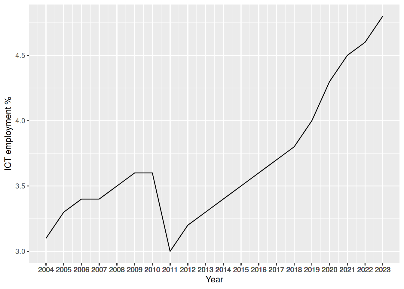
Breaks
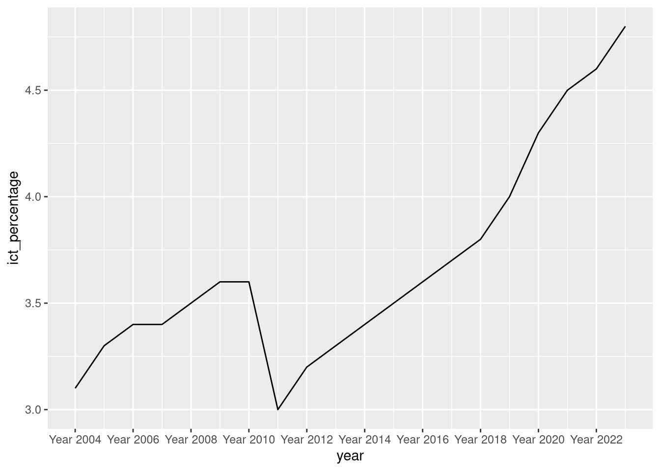
- In addition, if we want to modify the labels of the breaks, we can use the
labelsargument ofscale_x_continuous().
- Suppose, for example, that instead of having the years on the x-axis, we want to have labels formatted as
Year YYYY, whereYYYYis the year.
5.5 Breaks and their labels
5.6 Programming digression: creating sequences
- We have used the
seq()function to create the breaks and labels of the x-axis.
- The
seq()function creates sequences of numbers. - There are a few ways to create sequences in
R.
Programming digression: creating sequences
- The legacy way of creating sequences is to use the
:operator.
- The
:operator is used with infix notation. - It takes two arguments,
fromandto, and creates a sequence of integers fromfromtoto.
Programming digression: creating sequences
- The
:operator has a few disadvantages.
- First, it only works with a step of 1 or -1 if the
fromis smaller than theto. - Second, it can be error-prone when combined with arithmetic operations.
Programming digression: creating sequences
- A safer and more flexible way to create sequences is to use the
seq()function.
- The
seq()function can create sequences with an arbitrary step size.
Programming digression: creating sequences
- A safer and more flexible way to create sequences is to use the
seq()function.
- Or it can create sequences between two numbers with a specific length.
Programming digression: creating sequences
- A safer and more flexible way to create sequences is to use the
seq()function.
- Further, compared to the
:operator, there is less risk of confusion when combiningseq()with arithmetic operations.
Programming digression: creating sequences
- There are two very useful siblings of
seq(), namedseq_along()andseq_len().
Programming digression: creating sequences
- The
seq_along()function creates a sequence of integers from 1 to the length of the input vector.
- This is useful when we want to enumerate the elements of a vector.
Programming digression: creating sequences
- The
seq_len()function creates a sequence of integers from 1 to the input number.
- It gives the same result as
seq(1, 5).
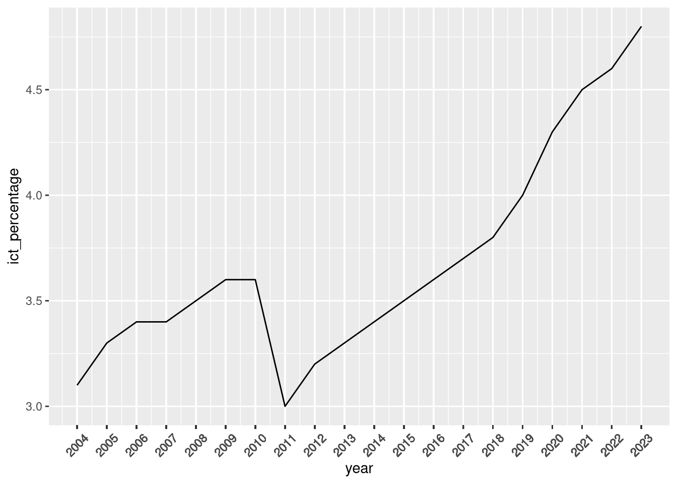
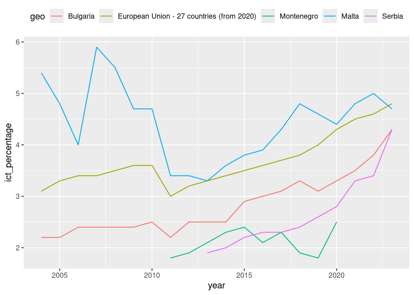
5.7 Rotating breaks’ labels
- When plotting high-frequency time-series data, the labels of the breaks on the horizontal axis can get crowded.
- One common way to address this issue is to rotate the labels.
- Rotating the labels does not affect the breaks or the labels themselves, only their orientation.
- We can rotate the breaks’ labels using the
theme()function.
Rotating breaks’ labels
- The
theme()function has (a lot of) options for modifying the plot’s theming.
- We can modify the appearance of the axes using the
axis.text.xandaxis.text.yarguments. - The
element_text()function is used to modify the appearance of the labels’ text. - Rotating the labels is done by setting the
angleargument to the desired angle (in degrees). - The
vjustandhjustarguments control the vertical and horizontal justification of the text.
Rotating breaks’ labels
5.8 Legends
- Another useful option exposed by
theme()is thelegend.positionargument.
Legends
- The
legend.positionargument can take the following values:"none": no legend is displayed."left","right","top","bottom": the legend is displayed on the left, right, top, or bottom of the plot area."inside": the legend is displayed inside the plot area.
Legends
- Besides customization via
theme(), legends can be modified using theguides()function.
- The
guides()function offers more fine-grained control over the appearance of the legend. - For example, we can modify the number of rows or columns of the legend.
- Or we can override the size and shape of the legend markers.
Legends
6 Statistical transformations
- How are data mapped to geometric objects?
- When creating a bar chart, we pass one column to
geom_bar(), and the function automatically calculates the height of the bars. - When creating a density plot, we pass one column to
geom_density(), and the function automatically calculates the density of the data.
6.1 Behind every geometric object
- How are data mapped to geometric objects?
- This pattern is common in
ggplot2. - The passed data is transformed into a new form that is used to create the plot.
- We examine some more details of the statistical transformations taking place behind the scenes when creating geometric objects.
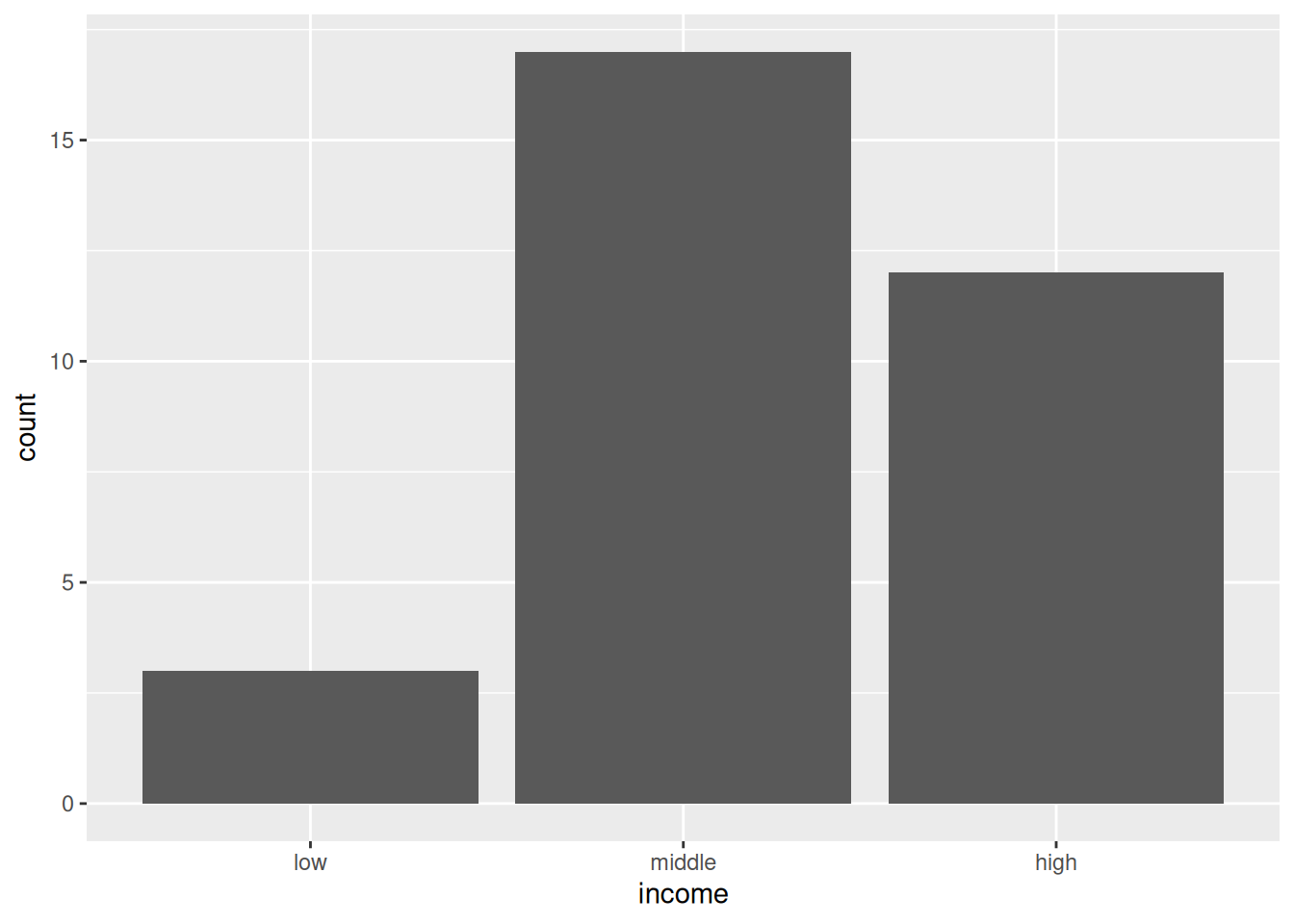
6.2 The statistic behind geom_bar()
- In the visualization overview topic, we created a bar chart of the income variable
eu_ict.

- Where is the
countvariable of the vertical axis coming from?
The statistic behind geom_bar()
- Where is the
countvariable of the vertical axis coming from?
- We have never defined
countas an aesthetic. - Even stranger,
countis not among the columns of theeu_ictdataset.
The statistic behind geom_bar()
- Examining the documentation of
geom_bar(), we observe that there is astatargument that defaults tocount.
Usage:
 geom_bar(
   mapping = NULL,
   data = NULL,
   stat = "count",
   position = "stack",
   ...,
   just = 0.5,
   width = NULL,
   na.rm = FALSE,
   orientation = NA,
   show.legend = NA,
   inherit.aes = TRUE
 )
The statistic behind geom_bar()
- Behind the scenes,
geom_bar()calculates the number of times each value ofincomeis found in the data.
- And then uses the new variable to set the heights.
The statistic behind geom_bar()
- We can manually replicate the calculation and instruct
geom_bar()not to perform any further transformation.
- Instructing a
geom_*function not to apply any statistical transformation to the input data is done by passingstat = "identity"to the function.
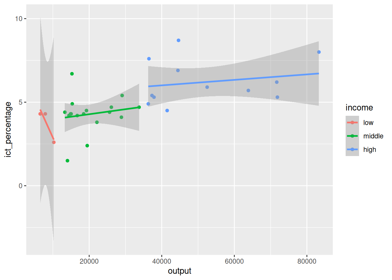
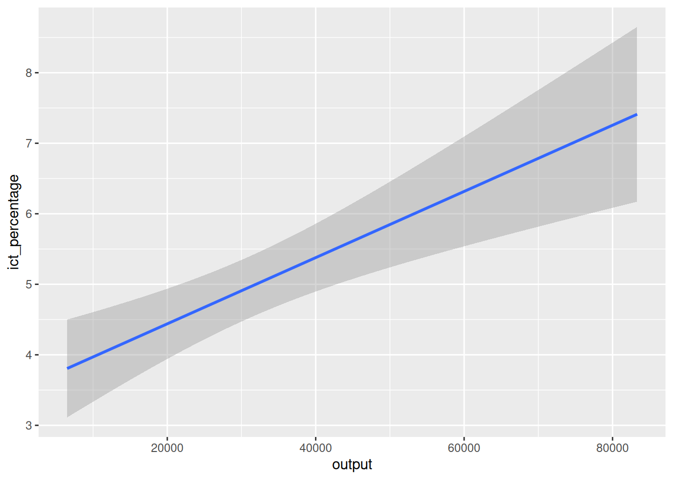
6.3 The statistics behind geom_smooth()
- Other
geom_*functions calculate different statistics by default.
- For instance,
geom_smooth()calculates fitted values, standard errors, and confidence intervals.
6.4 Programming digression: formulas
- How can we replicate the
geom_smooth()’s statistics?
- The
"lm"part of themethodargument stands for linear model. - Linear models are statistical models having linear relationships between the dependent and independent variables.
- For example, classic linear regressions are linear models.
Programming digression: formulas
- In
R, we have a neat way to define statistical models using formulas.
- Using formulas with
ggplot2and statistical functions allows us to focus on relationships in the data and leave the details of the statistical calculations to the functions.
Programming digression: formulas
A basic formula in
Rhas two main parts:- The left-hand side (LHS) of the formula is the dependent variable.
- The right-hand side (RHS) of the formula is the independent variable(s).
- The two parts are separated by a tilde
~symbol.
Programming digression: formulas
- Had we had more than one independent variable, we would have written:
- Note that we used the variables
ind_var1andind_var2in the formula, which neither were defined nor exist in any of our datasets. - And
Rdoes not complain about it.
Programming digression: formulas
- Had we had more than one independent variable, we would have written:
- This is because the formula does not actually calculate anything.
- It is an unevaluated expression that explains the logic of the model.
Linear regressions
- We can fit a linear model using formulas with the
lm()function.
- The first argument of
lm()is the formula we want to estimate. - The second argument is the dataset.
- The
lm()function automatically searches for the formula variables in the dataset and fits the model.
Linear regressions
Symbolically, we estimated the model,
\[ y_{i} = \beta_{0} + \beta_{1} x_{i} + \varepsilon_{i}, \]
- \(y_{i}\) is the
ict_percentage, - \(x_{i}\) is the
output, - \(\beta_{0}\) is the intercept,
- \(\beta_{1}\) is the slope, and
- \(\varepsilon_{i}\) is the error term.
- \(y_{i}\) is the
Linear regressions
How can we extract the predicted values from the model?
\[ \hat{y}_{i} = \hat{\beta}_{0} + \hat{\beta}_{1} x_{i} \]
Linear regressions
- How can we extract the confidence intervals?
\[ ce(\hat{y}_{i}) = [\hat{y}_{i} - t_{\alpha/2} \times \sigma(\hat{y}_{i}), \hat{y}_{i} + t_{\alpha/2} \sigma (\hat{y}_{i})] \]
where
\[ \sigma(\hat{y}_{i}) = \hat\sigma \sqrt{\frac{1}{n} + \frac{(x_{i} - \bar{x})^{2}}{\sum_{i=1}^{n} (x_{i} - \bar{x})^{2}}} \]
Linear regressions
- How can we extract the confidence intervals?
- When passing
interval = "confidence", thepredict()function returns a matrix with three columns:fit: the predicted values,lwr: the lower bound of the confidence interval, andupr: the upper bound of the confidence interval.
- We can examine the first few rows with
head().
Linear regressions
- How can we extract the confidence intervals?
- We can examine the first few rows with
head().
       fit      lwr      upr
1 5.277672 4.814736 5.740609
2 5.251859 4.792837 5.710880
3 3.871531 3.201614 4.541448
4 6.498425 5.648143 7.348707
5 4.865592 4.427362 5.303822
6 4.368092 3.852660 4.883525- We can now replicate the
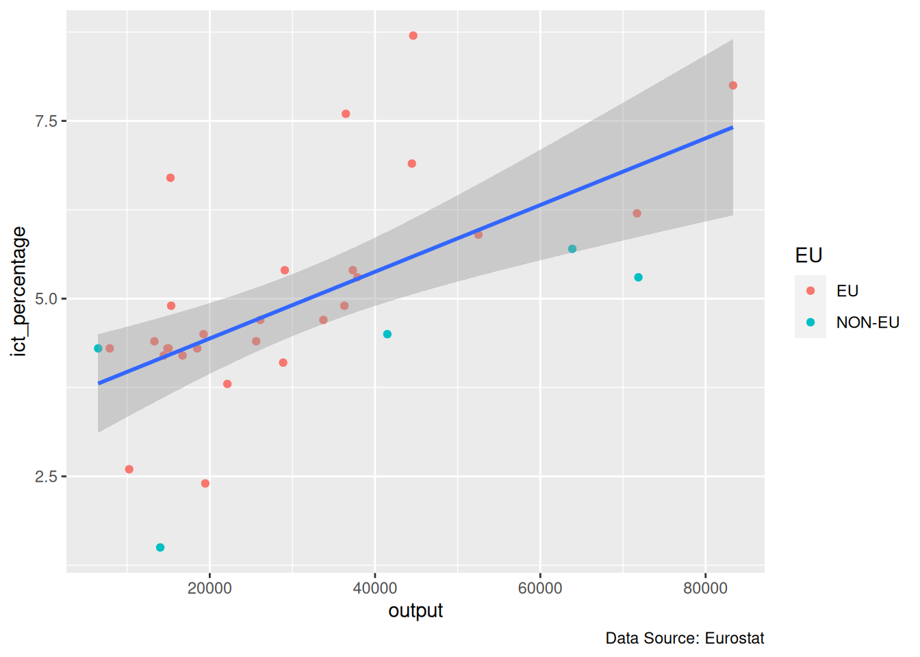
geom_smooth()’s statistics, and silence its noisy message about the formula use.
Linear regressions
fit <- lm(ict_percentage ~ output, eu_ict)
pred_y <- predict(fit, interval = "confidence")
eu_ict |>
  dplyr::mutate(
    pred = pred_y[, "fit"],
    ymin = pred_y[, "lwr"],
    ymax = pred_y[, "upr"]
  ) |>
  ggplot(aes(output)) +
  geom_line(aes(y = pred), color = "blue", linewidth = 1) +
  geom_ribbon(
    aes(ymin = ymin, ymax = ymax),
    fill = "darkgray",
    alpha = 0.5
  )

7 Text and annotations
- A common pattern in data science visualizations is the use of annotations and text.
- Text and annotations are commonly used to:
- Provide context
- Highlight specific data points
- Explain the data
- Add captions
7.1 Captions
- Captions can be effortlessly added to a figure with
labs().
Captions
Captions
7.2 Labels with Formulas
- On some occasions, data scientists want to include the underlying mathematical details of their work in a visualization.
- For example, suppose we are working with the function \[ f(x) = \sin(2x) + e^{-x/10} \cdot \cos(x) \]
- We can create a plot of \(f\) with
geom_line().
Labels with Formulas
\[ f(x) = \sin(2x) + e^{-x/10} \cdot \cos(x) \]
Labels with Formulas
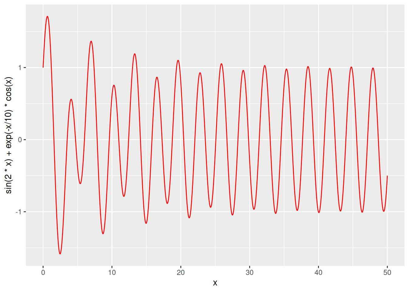
- Notice that
ggplot2writes the formula expression as a string in the vertical axis label.
- However, the used formatting is rather unusual for human readers.
- For instance, multiplication is denoted with
*, while in mathematical typography it is usually omitted.
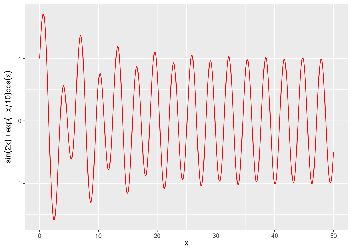
- We can use
quote()inlabs()to instructggplot2to render the expression in a more human-customary way.
Labels with Formulas
7.3 Annotations
- Besides captions and labels, we can add text and markers directly into the main body of the plot.
- These types of additions to a plot are called annotations.
- An annotation is an additional piece of information that is added to a plot and facilitates the interpretation of its data elements.
- In
ggplot2, annotations and text can be added withannotate()andgeom_text().
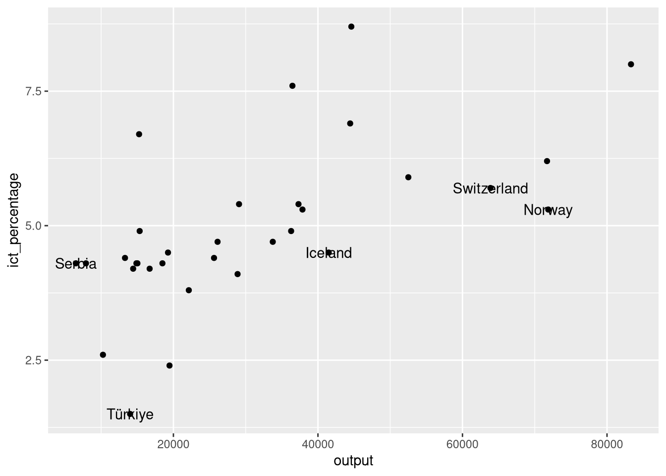
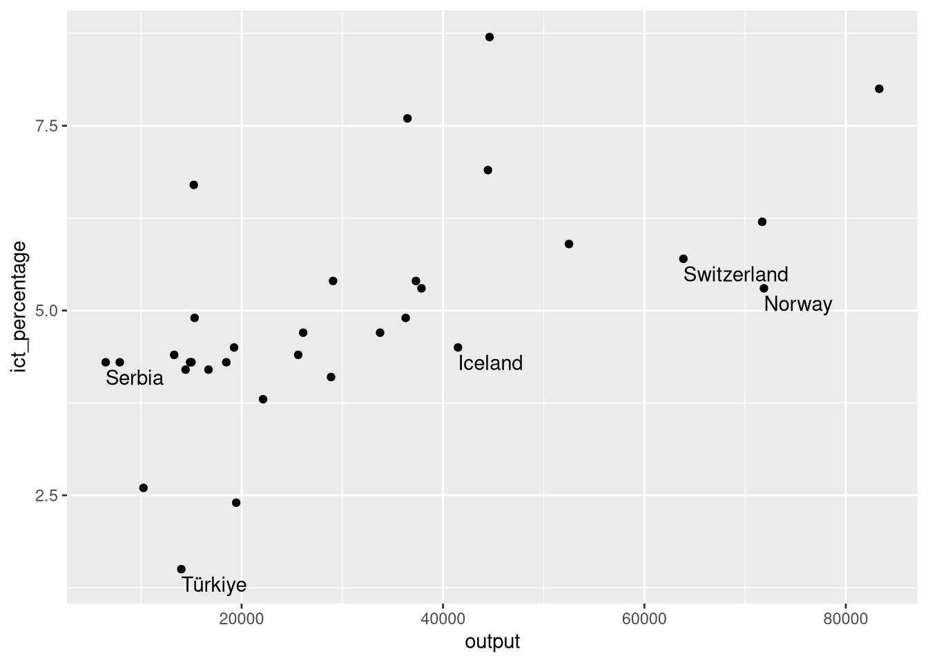
7.4 Using geom_text(): Example 1
- We want to textually highlight the non-EU countries in the
eu_ict’s scatter plot.

Using geom_text(): Example 1
- We want to textually highlight the non-EU countries in the
eu_ict’s scatter plot.

- We pass the
label = geoaesthetic togeom_text()to create a text object using country names.
- However, this creates a text object for all data points.
Using geom_text(): Example 1
- We want to textually highlight the non-EU countries in the
eu_ict’s scatter plot.
- We override the data argument of
geom_text()to filter only the non-EU countries.
- This looks more like what we want to achieve.
- Still, the text and the points are overlapping.
Using geom_text(): Example 1
- We want to textually highlight the non-EU countries in the
eu_ict’s scatter plot.

- We use
hjust = "left"andvjust = "top"to align the text to the top-left corner.
- Better, but some extra spacing could improve the aesthetics.
Using geom_text(): Example 1
- We want to textually highlight the non-EU countries in the
eu_ict’s scatter plot.
- We use
nudge_y = -0.1to move the text slightly below its data point.
Using geom_text(): Example 1
- We want to textually highlight the non-EU countries in the
eu_ict’s scatter plot.
- Finally, we can adjust the text size with the
sizeargument.
Using geom_text(): Example 1
- We want to textually highlight the non-EU countries in the
eu_ict’s scatter plot.

7.5 Using geom_text(): Example 2
- We want to textually highlight regression lines per group.
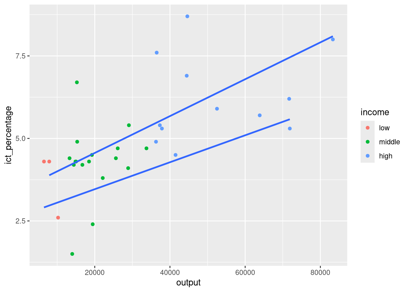
- Suppose we want to add the country names at the end of each regression line.
- We can pick the maximum
outputvalue per group and use it as thexaesthetic ingeom_text().
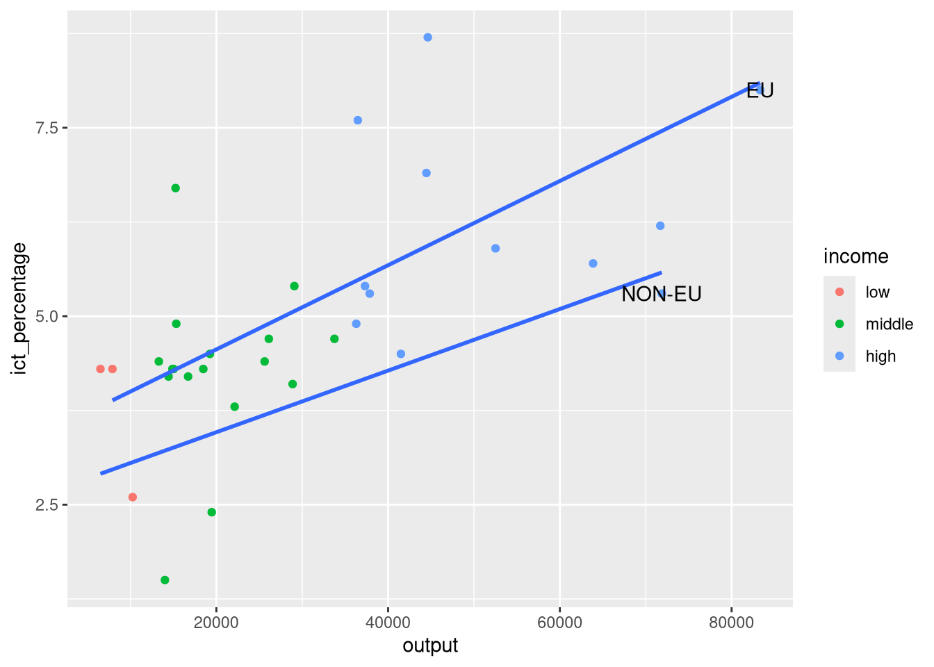
Using geom_text(): Example 2
- We want to textually highlight regression lines per group.
- We use
slice_max()to pick the maximumoutputvalue per group. - And override the data argument of
geom_text()to use the sliced data.
Using geom_text(): Example 2
- We want to textually highlight regression lines per group.
- We pass the aesthetics we want to use in the
mappingargument ofgeom_text().
Using geom_text(): Example 2
- We want to textually highlight regression lines per group.
ggplot(eu_ict, aes(output, ict_percentage)) +
  geom_point(aes(color = income)) +
  geom_smooth(
    aes(group = EU), method = "lm", se = FALSE, formula = y ~ x
) +
geom_text(
data = eu_ict |>
dplyr::group_by(EU) |>
dplyr::slice_max(output, n = 1),
aes(output, ict_percentage, label = EU),
hjust = "left",
vjust = "bottom",
nudge_x = 1000
)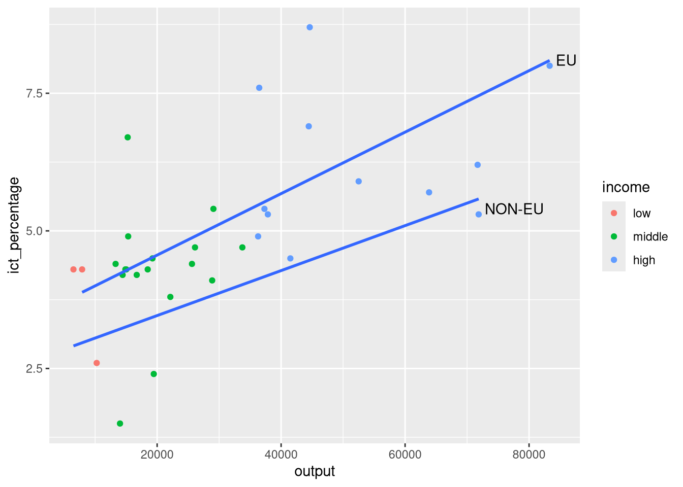
- And fine-tune the appearance of the text with
hjust,vjust, andnudge_x.
7.6 Annotating
- Another way to add text to a plot is with
annotate().
- In contrast to
geom_text(), which is a geometric object,annotate()does not act on data points. - This means that
annotate()does not require a data argument. - And it is more useful for adding small, data-independent elements to a plot.
7.7 Using annotate() for text
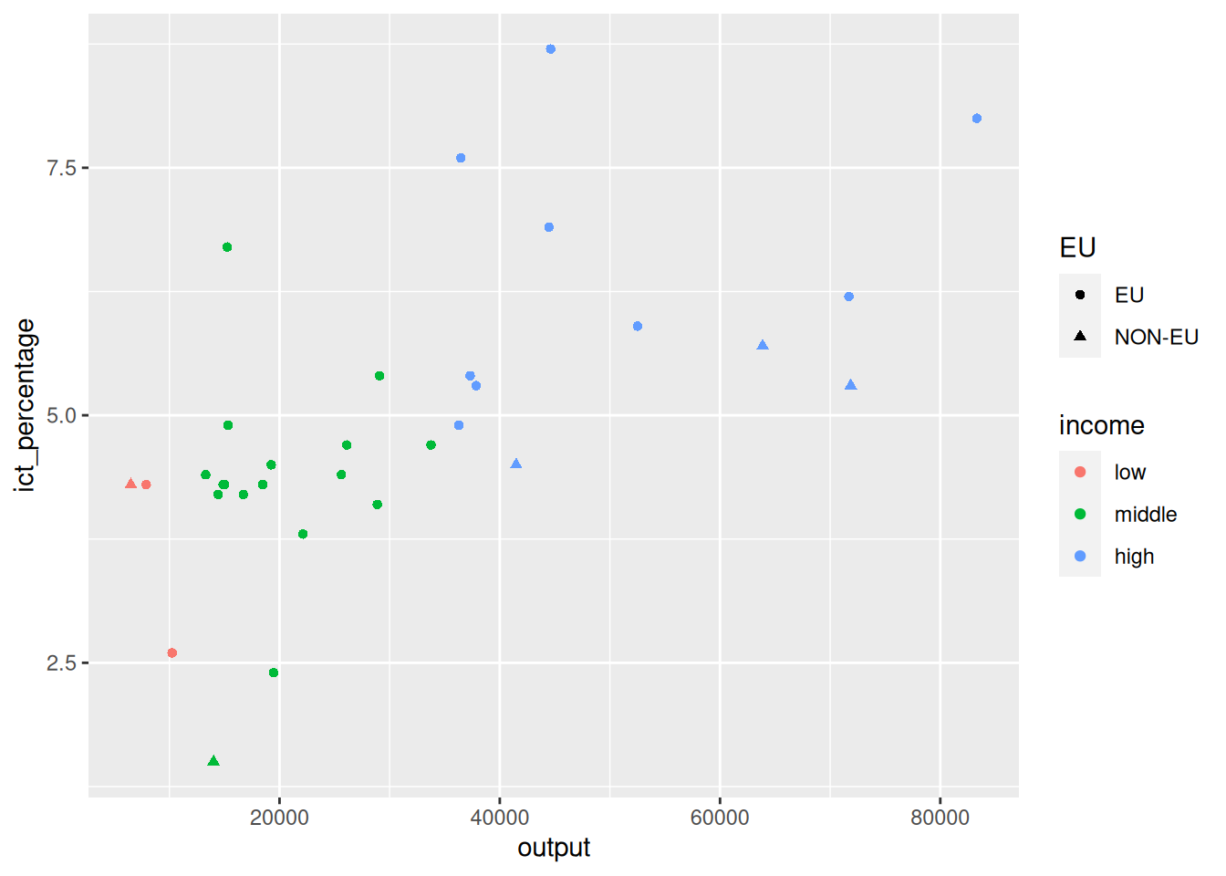
- We want to add a label next to the richest EU country.
- We start once more with a
geom_point()scatter plot of theeu_ict’sincomedata.
Using annotate() for text
- We want to add a label next to the richest EU country.
Using annotate() for text
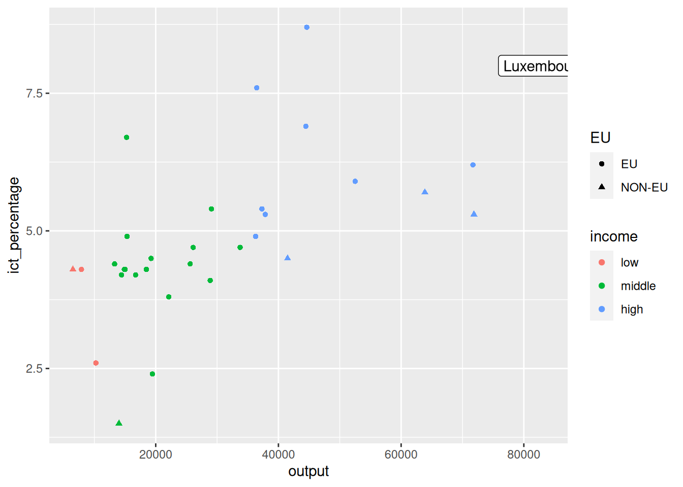
- We want to add a label next to the richest EU country.
- And add an
annotate()of geometric typelabel.
- On its own, this gives an error if executed.
- We need to provide the
labeltext for the annotation. - And specify the position for the label using the
xandyarguments.
Using annotate() for text
- We want to add a label next to the richest EU country.
- We can do some preliminary data transformations to find the richest EU country.
Using annotate() for text
- We want to add a label next to the richest EU country.
- And use the calculated
richestdata to pass more information toannotate().
Using annotate() for text
- We want to add a label next to the richest EU country.
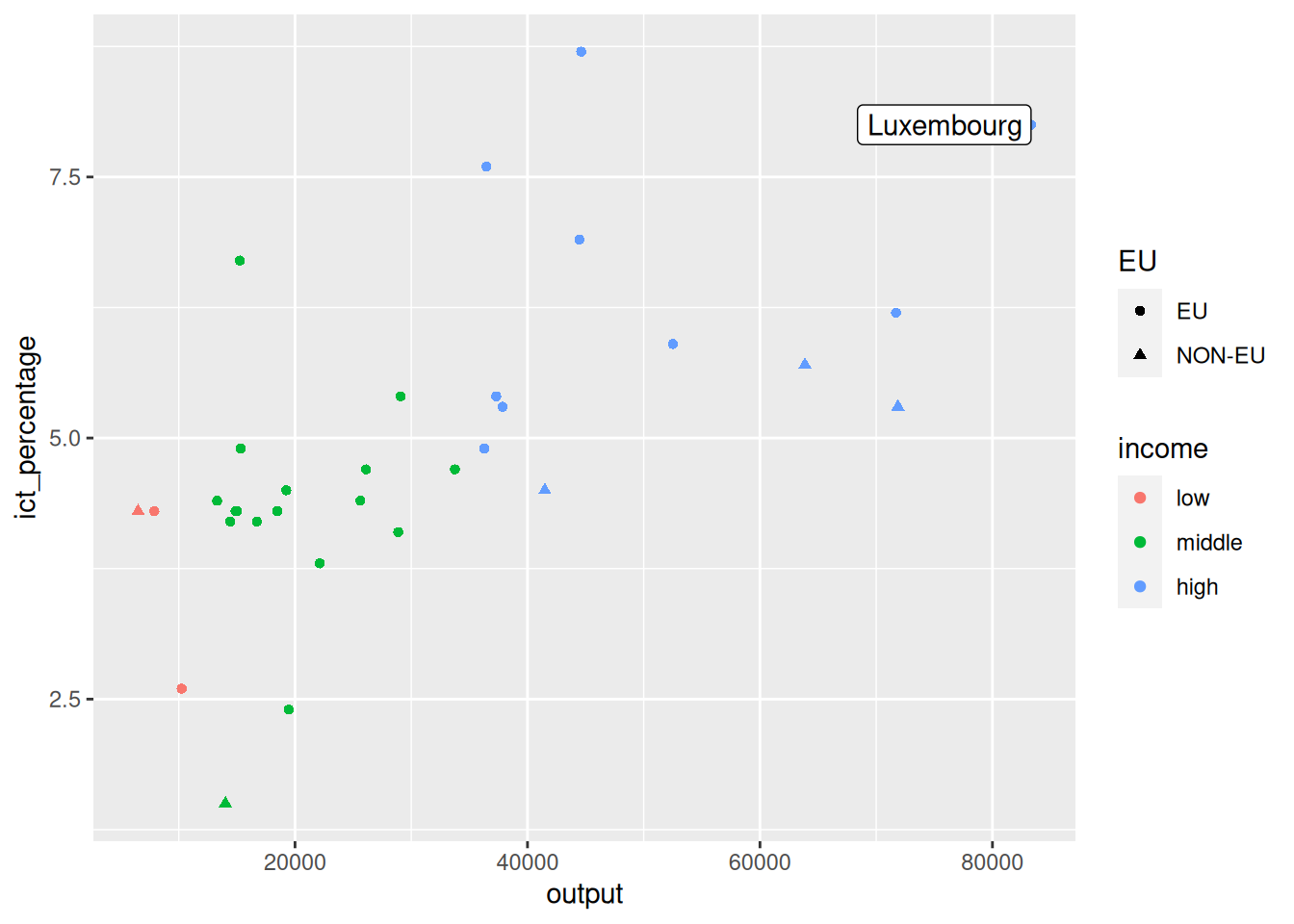
- We can adjust the label’s text horizontal alignment.
Using annotate() for text
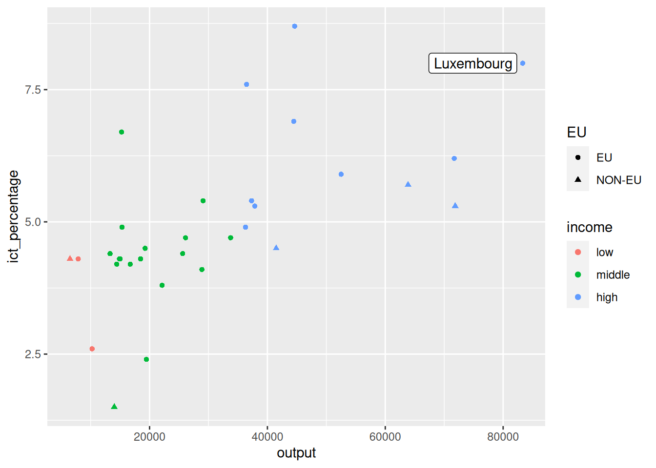
- We want to add a label next to the richest EU country.
- The
annotate()function does not havenudge_*arguments (why?).
- We can directly adjust the
xandypositions to move the label around.
Using annotate() for text
- We want to add a label next to the richest EU country.
Using annotate() for text
7.8 Using annotate() for segments
- Using
annotate()is very useful for adding segments and arrows to a plot.
- The calling interface is mostly similar to
annotate()for text. - Instead of
geom = "label", we usegeom = "segment"to create annotations with segments and arrows.
Using annotate() for segments
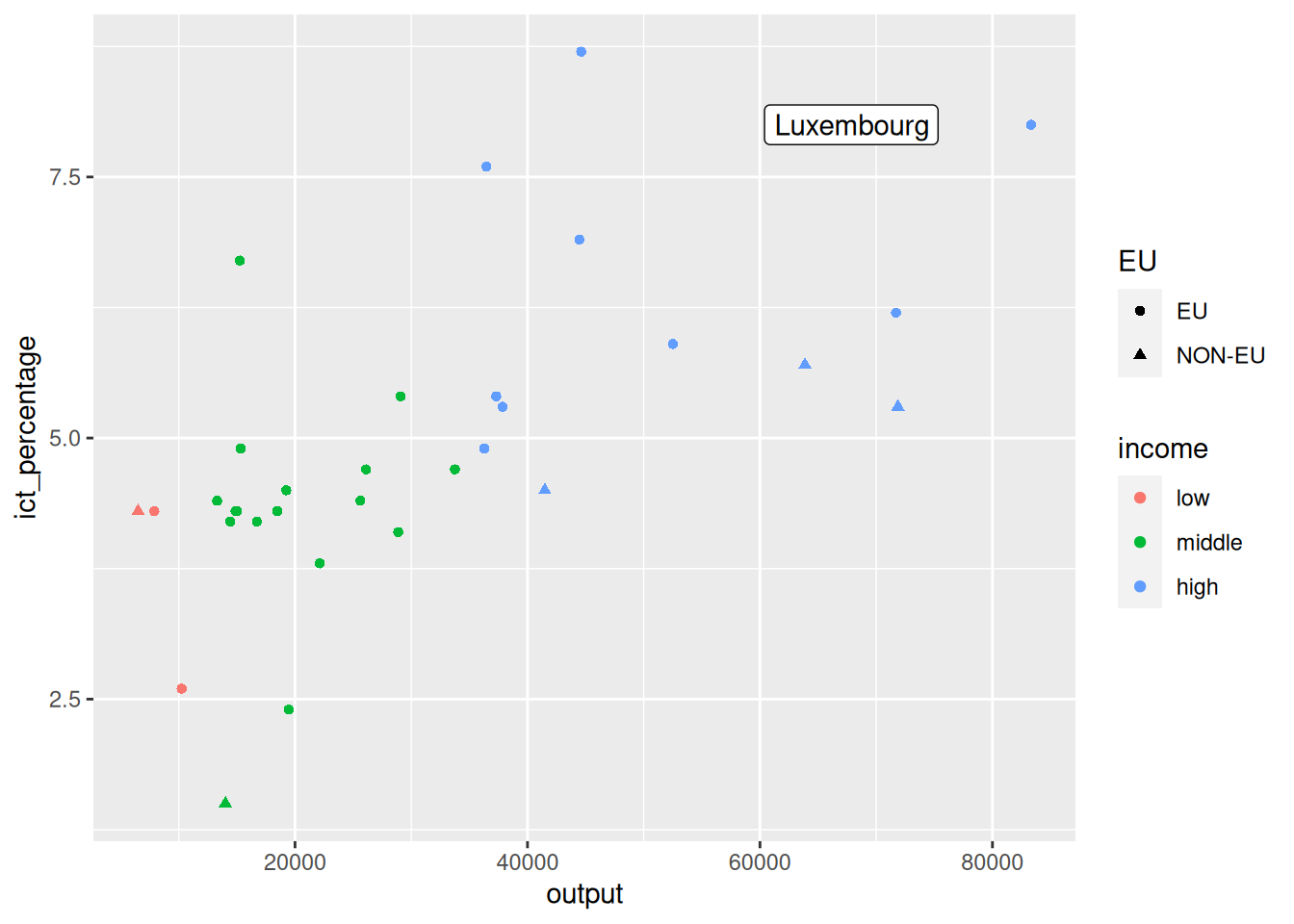
- We nudge the label of the richest country a bit more to the left.
Using annotate() for segments
richest <- eu_ict |>
dplyr::filter(EU == "EU") |>
dplyr::slice_max(output, n = 1)
ggplot(eu_ict, aes(output, ict_percentage)) +
geom_point(aes(color = income, shape = EU)) +
annotate(
geom = "label",
label = richest$geo,
x = richest$output - 8000,
y = richest$ict_percentage,
hjust = "right"
) +
annotate(geom = "segment")- And add a new
annotate()layer withgeom = "segment"to create a segment.
Using annotate() for segments
richest <- eu_ict |>
  dplyr::filter(EU == "EU") |>
  dplyr::slice_max(output, n = 1)
ggplot(eu_ict, aes(output, ict_percentage)) +
  geom_point(aes(color = income, shape = EU)) +
  annotate(
    geom = "label",
    label = richest$geo,
    x = richest$output - 8000,
    y = richest$ict_percentage,
    hjust = "right"
) +
annotate(geom = "segment")- Specifying a segment on a plane is equivalent to specifying two points.
- The
annotate()function expects two points to draw the segment. - The points are specified by the
x,y,xend, andyendarguments.
Using annotate() for segments
richest <- eu_ict |>
  dplyr::filter(EU == "EU") |>
  dplyr::slice_max(output, n = 1)
ggplot(eu_ict, aes(output, ict_percentage)) +
  geom_point(aes(color = income, shape = EU)) +
  annotate(
    geom = "label",
    label = richest$geo,
    x = richest$output - 8000,
    y = richest$ict_percentage,
    hjust = "right",
  ) +
  annotate(
    geom = "segment",
    x = richest$output - 8000,
    xend = richest$output - 500,
    y = richest$ict_percentage,
    yend = richest$ict_percentage
  )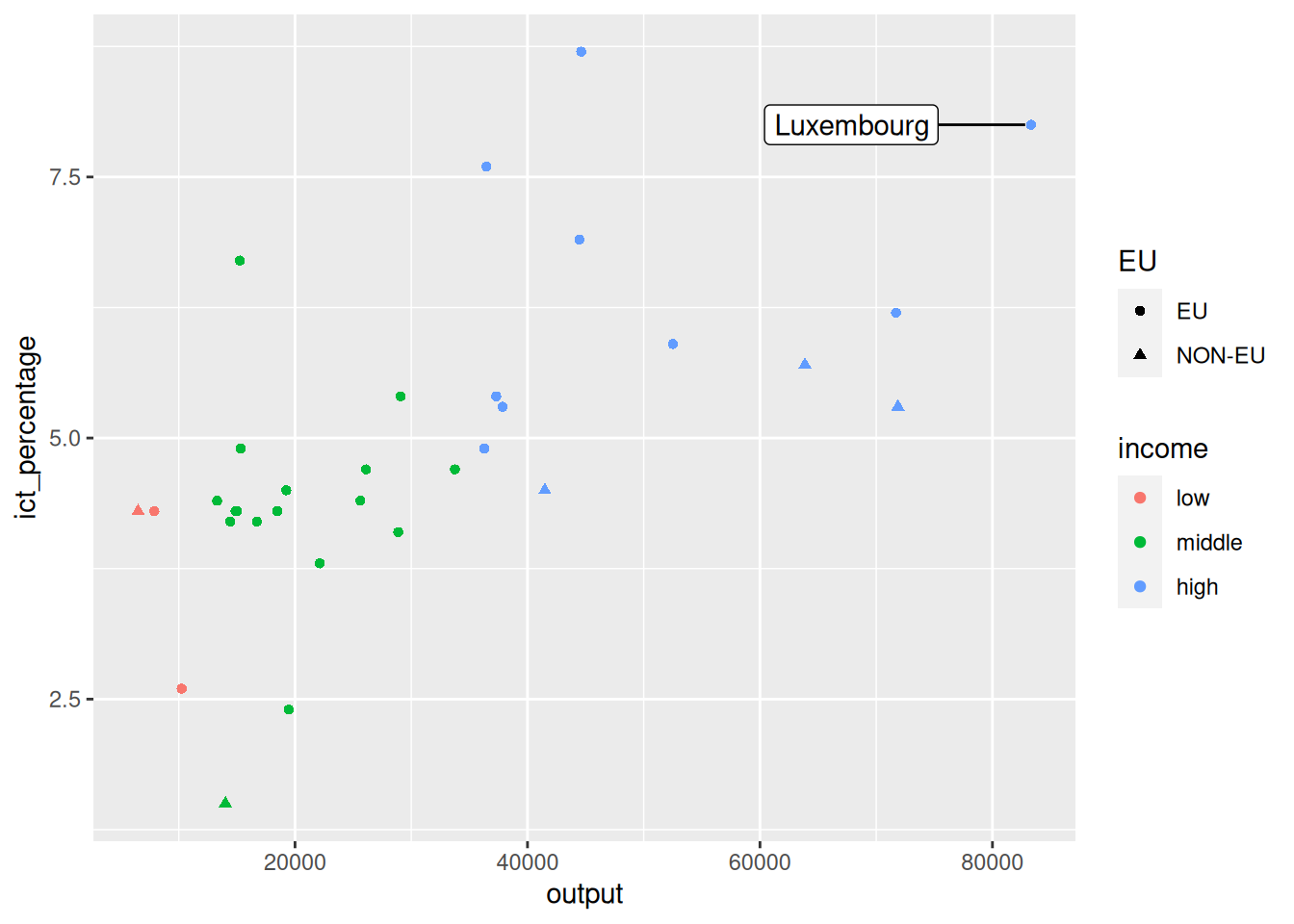
- This creates a segment connecting the two points, but not an arrowhead.
Using annotate() for segments
richest <- eu_ict |>
  dplyr::filter(EU == "EU") |>
  dplyr::slice_max(output, n = 1)
ggplot(eu_ict, aes(output, ict_percentage)) +
  geom_point(aes(color = income, shape = EU)) +
  annotate(
    geom = "label",
    label = richest$geo,
    x = richest$output - 8000,
    y = richest$ict_percentage,
    hjust = "right",
  ) +
  annotate(
    geom = "segment",
    x = richest$output - 8000,
    xend = richest$output - 500,
    y = richest$ict_percentage,
    yend = richest$ict_percentage,
    arrow = arrow(type = "closed", length = unit(0.3, "cm"))
)![]()
- We can add an arrowhead to the plot using the
arrowargument.
Using annotate() for segments
richest <- eu_ict |>
  dplyr::filter(EU == "EU") |>
  dplyr::slice_max(output, n = 1)
ggplot(eu_ict, aes(output, ict_percentage)) +
  geom_point(aes(color = income, shape = EU)) +
  annotate(
    geom = "label",
    label = richest$geo,
    x = richest$output - 8000,
    y = richest$ict_percentage,
    hjust = "right",
  ) +
  annotate(
    geom = "segment",
    x = richest$output - 8000,
    xend = richest$output - 500,
    y = richest$ict_percentage,
    yend = richest$ict_percentage,
    arrow = arrow(type = "closed", length = unit(0.3, "cm")),
    color = "red"
  )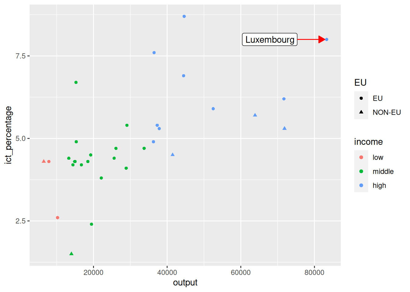
- Finally, the color of the annotation can be adjusted with the
colorargument.