Coding & Data Visualization with Generative AI

Last Updated: July 15th, 2026
Impact of Generative AI on Productivity
Cui et al. (2024) studied the impact of generative AI on productivity.

Who benefits the most?
Cui et al. (2024) studied the impact of generative AI on productivity.

Install R extension

Install R extension

Install R extension
Install languageserver

Install languageserver

Install languageserver

Install Copilot extension
Install Copilot extension

Install Copilot extension
Create course folder codv

Create source file overview.R
Create source file overview.R

Install tidyverse

Install tidyverse

An empty canvas
- We start by creating an empty canvas for the visualization.
Adding Axes

Adding Axes
Adding a scatter plot
- We aim to add a scatter plot on the canvas.

Coloring the points
- We aim to colorize the points based on the EU membership.

Adding curves
- We aim to add linearly fitted lines to the scatter plot.

Adding a single curve
- We aim to add a single linearly fitted line to the scatter plot.
- The last code chunk respected the coloring aesthetics we defined earlier.
- What if we want to add a single fitted line to the scatter plot?
Adding a single curve
- We aim to add a single linearly fitted line to the scatter plot.

Adding shape aesthetics
- We aim to reshape point markers based on a categorical variable.
- On some occasions, differentiating points based on colors might not be enough (e.g., printing in black and white).
Adding shape aesthetics
- We aim to reshape point markers based on a categorical variable.
- Instead, we can use different shapes to represent different categories.
- Or, we can combine both color and shape aesthetics.
Adding shape aesthetics
- We aim to reshape point markers based on a categorical variable.

Adding titles and labels
- We aim to display some text information on the plot.
ggplot(
  data = eu_ict,
  mapping = aes(x = output, y = ict_percentage)
) +
geom_point(mapping = aes(color = EU, shape = EU)) +
geom_smooth(method = "lm") +
labs(
title = "ICT employment and Output",
subtitle = "EU27 vs. non-EU27 countries",
x = "Output per capita (EUR)",
y = "ICT employment (percentage of total employment)",
color = "Membership",
shape = "Membership"
)
Color scaling
- We aim to recolor the figure in grayscale.
ggplot(
  data = eu_ict,
  mapping = aes(x = output, y = ict_percentage)
) +
geom_point(mapping = aes(color = EU, shape = EU)) +
geom_smooth(method = "lm") +
labs(
title = "ICT employment and Output",
subtitle = "EU27 vs. non-EU27 countries",
x = "Output per capita (EUR)",
y = "ICT employment (percentage of total employment)",
color = "Membership",
shape = "Membership"
) +
scale_color_grey()
- The
scale_color_grey()function did not recolor the fitted line (why?). - We can manually set the color of the fitted line.
Color scaling
- We aim to recolor the figure in grayscale.
ggplot(
  data = eu_ict,
  mapping = aes(x = output, y = ict_percentage)
) +
geom_point(mapping = aes(color = EU, shape = EU)) +
geom_smooth(method = "lm", color = "darkgray") +
labs(
title = "ICT employment and Output",
subtitle = "EU27 vs. non-EU27 countries",
x = "Output per capita (EUR)",
y = "ICT employment (percentage of total employment)",
color = "Membership",
shape = "Membership"
) +
scale_color_grey()
A first bar plot
- We wish to create a bar plot of the
incomevariable in theeu_ictdataset.

- The
incomevariable is categorical and has three levels:low,middle, andhigh.
- The levels are depicted on the axis used in the
aes()call.
- The other axis depicts the number of observations in each level.
Histograms of continuous variables
- We aim to create a histogram of the (continuous)
outputvariable.

- In contrast to categorical variables, for which the number of bins is determined by the number of levels, histograms of continuous variables can be created with different numbers of bins.
Histograms of continuous variables
- We aim to create a histogram of the (continuous)
outputvariable.
- By default, the
geom_histogram()function uses 30 bins.
- This might not be what we want.
Histograms of continuous variables
- We aim to create a histogram of the (continuous)
outputvariable.

Density plots
- An alternative way to visualize the distribution of a continuous variable is to use a density plot.

Density plots
- Unlike the histogram case, the vertical axis of the density plot does not measure frequencies of observations.
- Very roughly, one can think of the density plots as having smoothed-out values of the number of observations over bins with tiny widths.
- These values can be greater or smaller than 1.
Ordering bar plots levels
- We need to load the
forcatspackage to use these functions.

Coloring bar plots
- Let us plot the distribution of
incomelevels byeucountries in theeu_ictdataset.

Coloring bar plots
- Let us plot the distribution of
incomelevels byeucountries in theeu_ictdataset.

Coloring bar plots
- Let us plot the distribution of
incomelevel shares byeucountries in theeu_ictdataset.
- One issue with the last plot is that splitting countries based on
EUmembership is very unbalanced.
Coloring bar plots
- Let us plot the distribution of
incomelevel shares byeucountries in theeu_ictdataset.
- There are many more
EUcountries thanNON-EUcountries in the dataset, making comparisons challenging.
Coloring bar plots
- Let us plot the distribution of
incomelevel shares byeucountries in theeu_ictdataset.
- We can ask
ggplot2to normalize the bar heights and color by theincomeshares within eachEUmembership category.
Coloring bar plots
- We would like to plot the distribution of
incomelevel shares byeucountries in theeu_ictdataset.

Coloring density plots
- We would like to plot the distributions of
ict_percentageperincomegroup.

- We can further highlight the plot’s densities by using a
fillaesthetic instead of or alongsidecolor.
Coloring density plots
- We would like to plot the distributions of
ict_percentageperincomegroup.

- We can make the plot easier to read by using a
fillaesthetic instead of or alongsidecolor.
- However, with overlapping densities, it is difficult to distinguish the density shape of each group.
Coloring density plots
- We would like to plot the distributions of
ict_percentageperincomegroup.
- We can pass an
alpha(transparency) value to thegeom_density()function to make the plot more readable.
Coloring density plots
- We would like to plot the distributions of
ict_percentageperincomegroup.

- We can pass an
alpha(transparency) value to thegeom_density()function to make the plot more readable.
- The
alphavalue ranges from 0 (completely transparent) to 1 (completely opaque).
Visualizing box plots
- We want to concisely visualize the basic statistics of
ict_percentageperincomegroup.

Visualizing box plots
- The median is displayed as a solid horizontal line inside each box.
- The first and third quartiles are displayed as the lower and upper edges of each box.
- Whiskers indicate the range of non-outlier values.
- Outliers are displayed as individual points.
- Skewness is indicated by the position of the median relative to the quartiles.
The limits of ekphrasis
- In some sense, data science activities are a form of art.
- A good statistic and its visualization can convey a message and reveal a pattern more effectively than an endless stream of numbers and text.
- In most ways, however, data science is very different from (at least surreal forms of) art.
- It has to be grounded and faithful to the data it represents.
- Unfortunately, governments, academics, and companies sometimes use more than recommended poetic freedom.

Misrepresenting the addiction risk

Misrepresenting the addiction risk
Argentinian inflation statistics

Source: Aragão and Linsi (2022)
Overview
- There are many IDEs with varying feature sets.

More than a text editor
- The (development) process of editing, translating, executing, and debugging was repeated until the program was working as expected.
- During these iterations, one had to switch between different environments and tools many times.
- The idea of IDEs is to integrate all needed tools in a single environment to increase productivity.

Modern IDEs
- For \(L\) languages and \(I\) IDEs, every feature had to be implemented \(L \times I\) times.

Why was it so successful?
- By specifying the communication rules, the LSP reduces the \(L \times I\) to an \(L + I\) implementation problem.

Why was it so successful?
- Programming languages implement language servers that understand the LSP.
- IDEs implement clients that understand the LSP.
- No need for feature implementation duplication.
Reproducibility


Programming digression: R namespaces
- Organizing and managing function and object names in namespaces is a way to avoid conflicts between different modules.

Programming digression: set operations
- The order of the arguments is important in this case because the set difference operation is not symmetric.

Programming digression: set operations
- We use the
intersect()function to find the common elements of two vectors.
- Unlike
setdiff(), the order of the arguments does not matter because the intersection operation is symmetric.

Programming digression: set operations
- To get the combination of unique values, we use
union().
- Unions are symmetric, so any order of the arguments gives the same elements.
- The order of the elements can be different, though.

Data Colada

Simonsohn, Nelson, and Simmons (2023)
Data Colada

Simonsohn, Nelson, and Simmons (2023)
Exact matching
- By exact matching.

Partial matching
- By partial matching.


Positional arguments
- By position

Positional arguments
- The same applies to the
aes()function.

Defining aesthetics
- Aesthetics can be defined at various levels when creating a plot.

Defining aesthetics
- Aesthetics can be defined at various levels when creating a plot.

Defining aesthetics
- Aesthetics can be defined at various levels when creating a plot.

Defining aesthetics: how
- How does this work?

Defining aesthetics: why


Defining aesthetics
- Why does it work in this way?

Basic themes

Basic themes
Basic themes
- We can apply themes to the plot by adding them with the
+operator.


Basic themes
- Themes only affect the non-data elements of the plot.
Basic themes
- Themes only affect the non-data elements of the plot.

Basic themes
- Themes only affect the non-data elements of the plot.
- Here, we have combined the
theme_bw()withscale_color_grey()to modify the appearance of the data elements. - In addition, we have explicitly specified the color of the
geom_smooth()object to be black.
Additional themes
- The
ggthemespackage provides additional themes that might match the desired style.

Labels

Labels
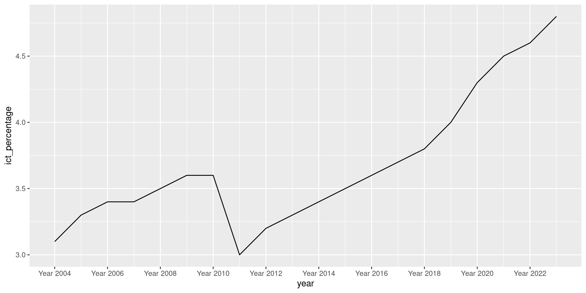
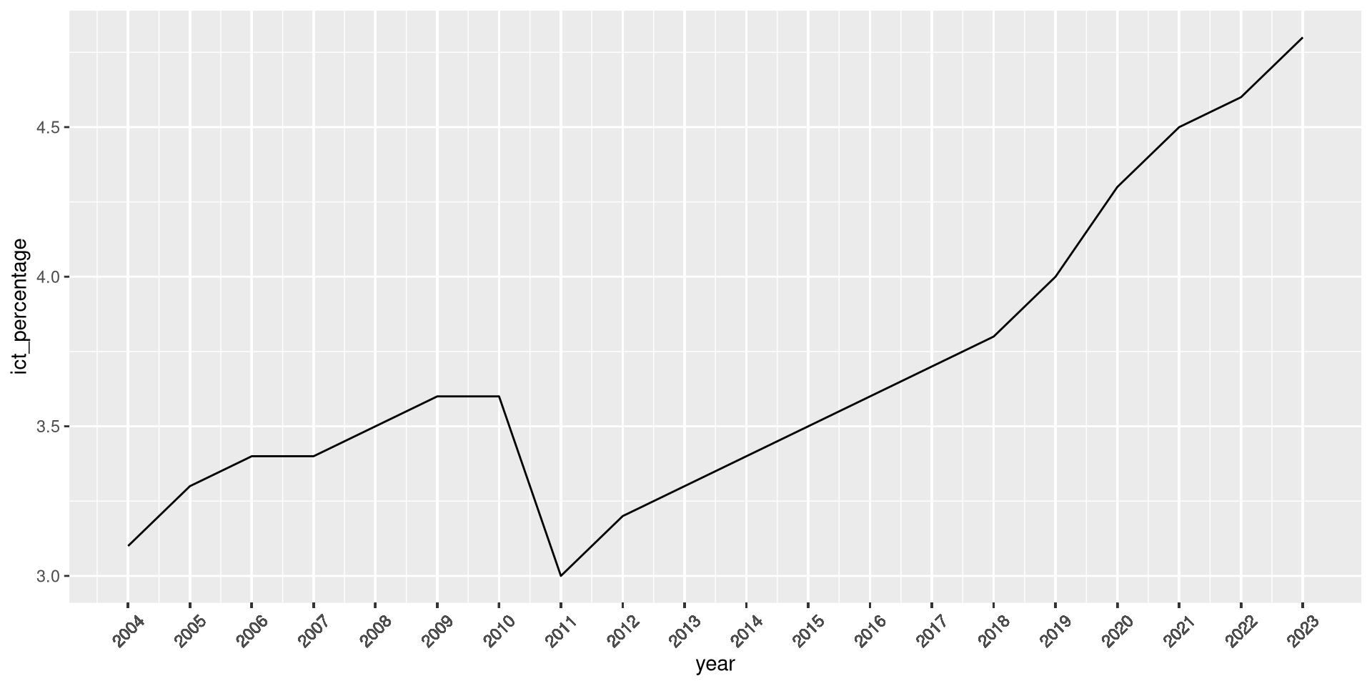
Breaks

- We can pass directly the breaks we want to have on a continuous axis using the
breaksargument.
- For instance, if we want to have all the years as breaks, we can pass the
yearcolumn of theictdata frame.
Breaks

Breaks and their labels
Rotating breaks’ labels
Legends
- Another useful option exposed by
theme()is thelegend.positionargument.
Legends
The statistic behind geom_bar()
- In the visualization overview topic, we created a bar chart of the income variable
eu_ict.

- Where is the
countvariable of the vertical axis coming from?
The statistic behind geom_bar()
- We can manually replicate the calculation and instruct
geom_bar()not to perform any further transformation.
- Instructing a
geom_*function not to apply any statistical transformation to the input data is done by passingstat = "identity"to the function.

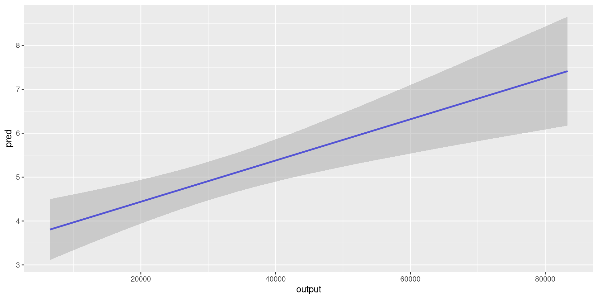
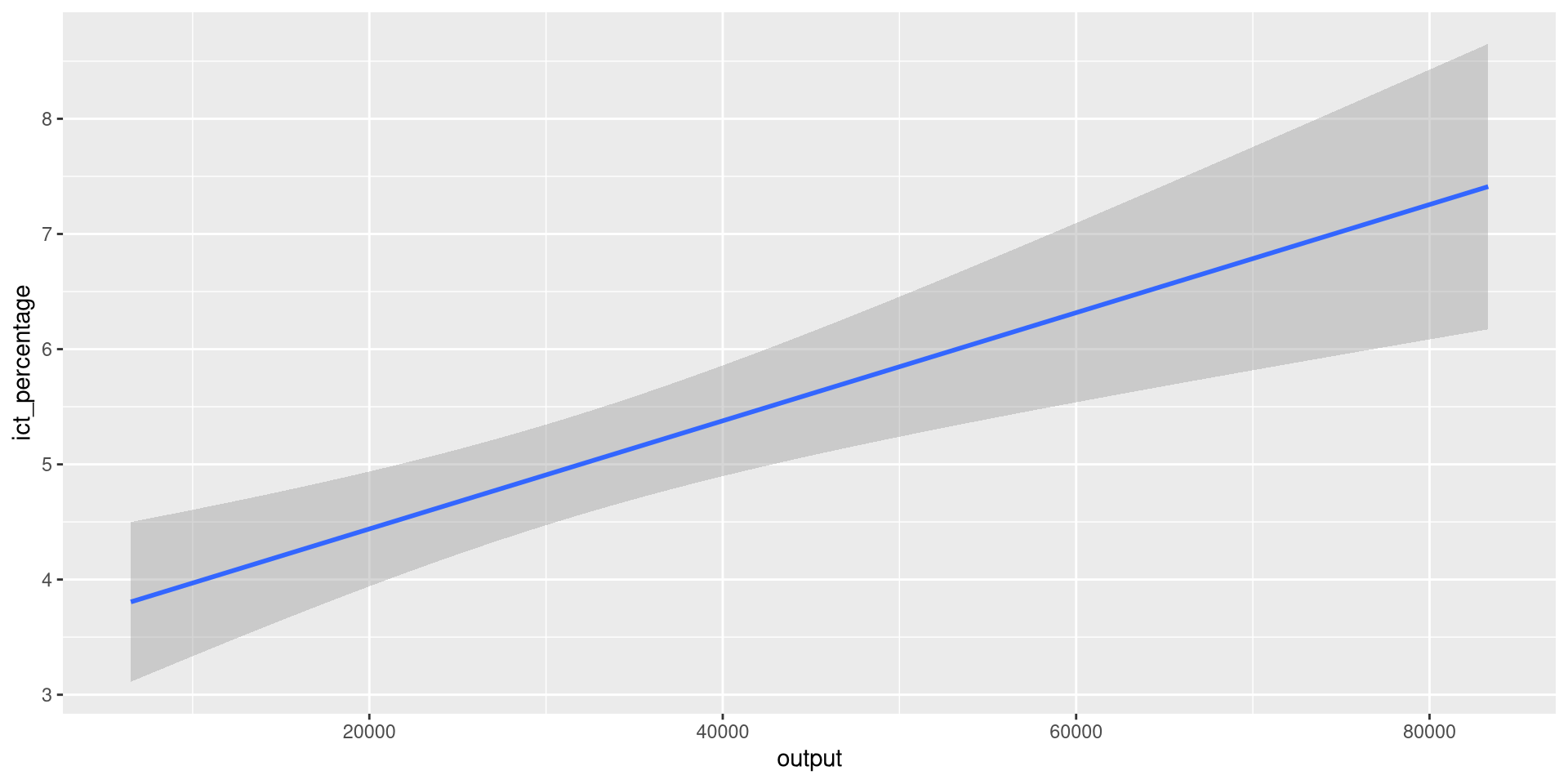
The statistics behind geom_smooth()
- Other
geom_*functions calculate different statistics by default.
- For instance,
geom_smooth()calculates fitted values, standard errors, and confidence intervals.

Linear regressions
fit <- lm(ict_percentage ~ output, eu_ict)
pred_y <- predict(fit, interval = "confidence")
eu_ict |>
dplyr::mutate(
pred = pred_y[, "fit"],
ymin = pred_y[, "lwr"],
ymax = pred_y[, "upr"]
) |>
ggplot(aes(output)) +
geom_line(aes(y = pred), color = "blue", linewidth = 1) +
geom_ribbon(
aes(ymin = ymin, ymax = ymax),
fill = "darkgray",
alpha = 0.5
)
Captions

Captions
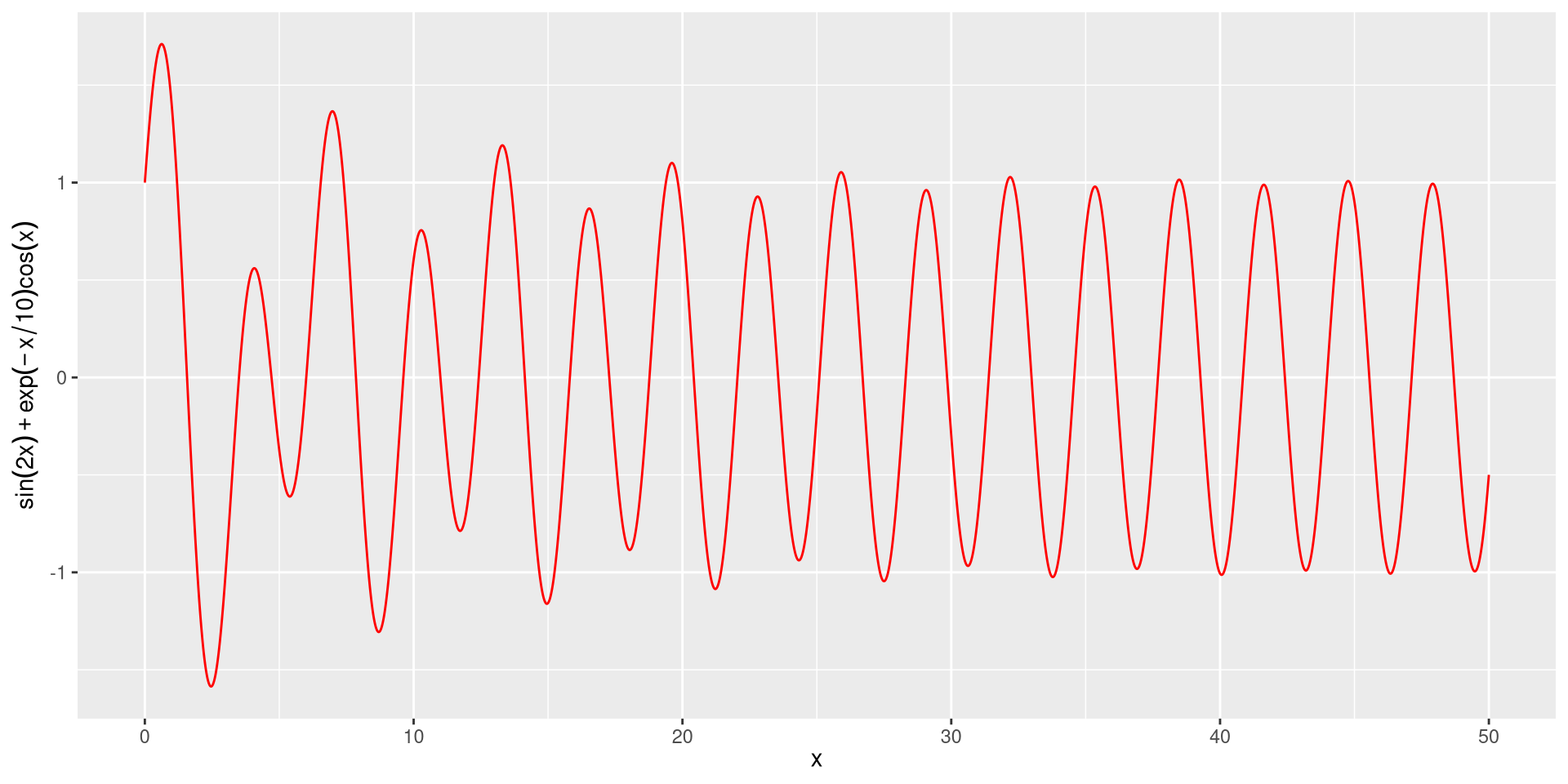
Labels with Formulas
\[ f(x) = \sin(2x) + e^{-x/10} \cdot \cos(x) \]
Labels with Formulas

- Notice that
ggplot2writes the formula expression as a string in the vertical axis label.
- However, the used formatting is rather unusual for human readers.
- For instance, multiplication is denoted with
*, while in mathematical typography it is usually omitted.
- We can use
quote()inlabs()to instructggplot2to render the expression in a more human-customary way.
Labels with Formulas
Using geom_text(): Example 1
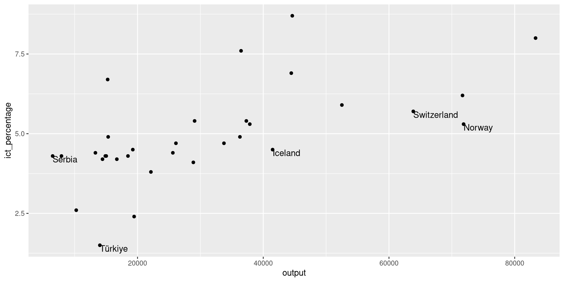
- We want to textually highlight the non-EU countries in the
eu_ict’s scatter plot.

Using geom_text(): Example 1
- We want to textually highlight the non-EU countries in the
eu_ict’s scatter plot.
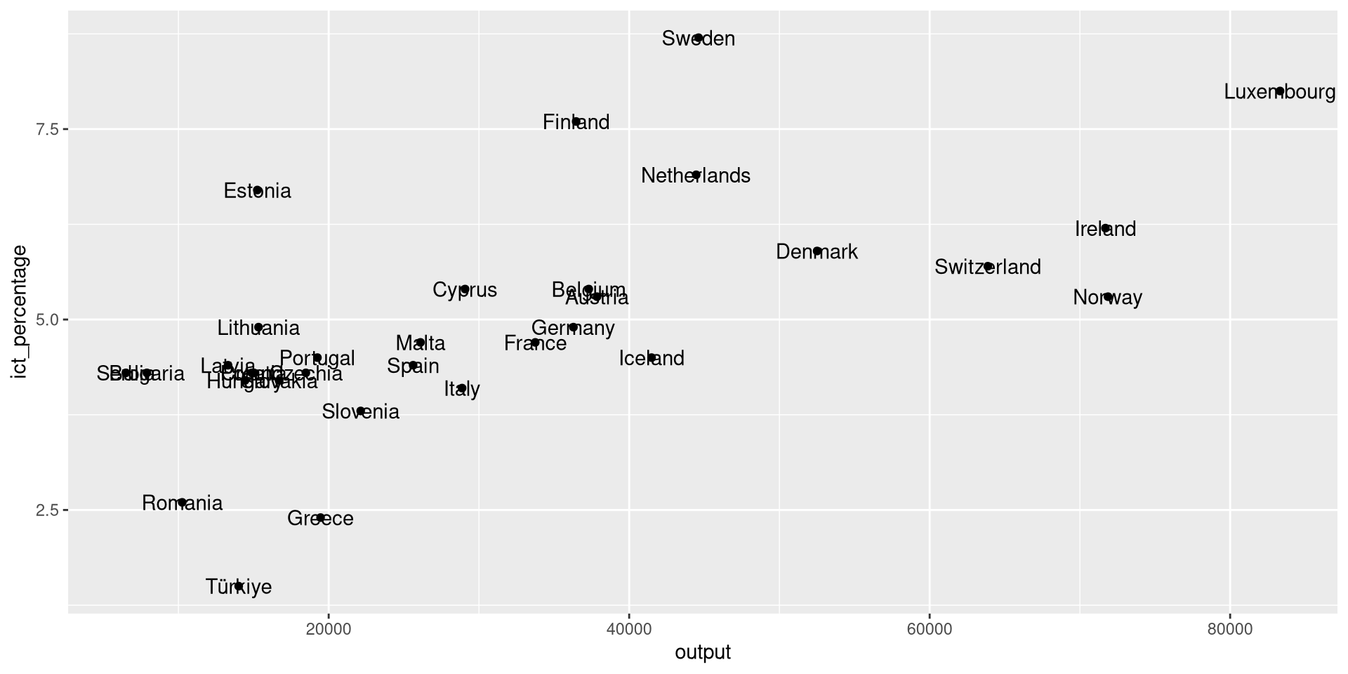
- We pass the
label = geoaesthetic togeom_text()to create a text object using country names.
- However, this creates a text object for all data points.
Using geom_text(): Example 1
- We want to textually highlight the non-EU countries in the
eu_ict’s scatter plot.
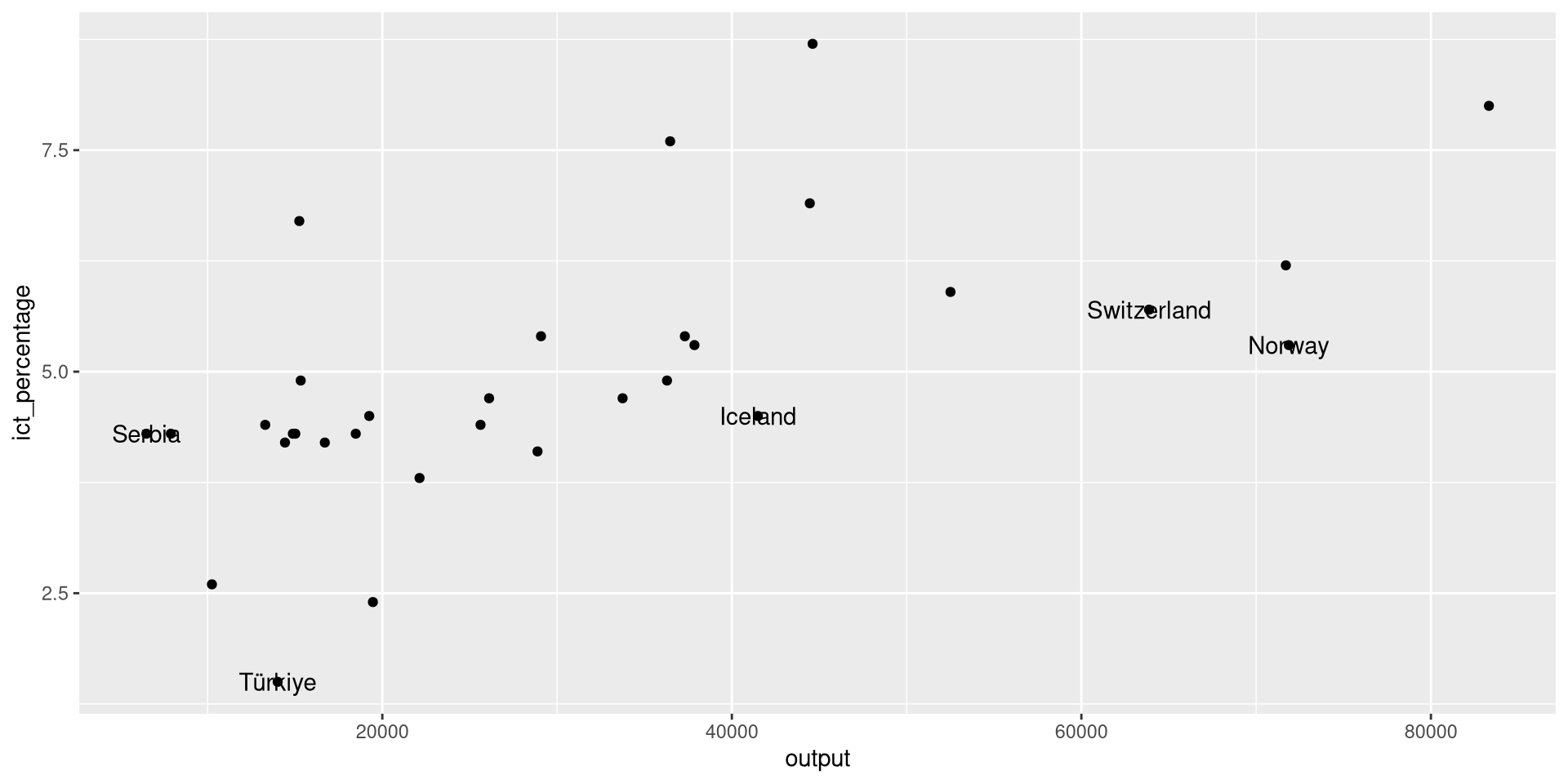
- We override the data argument of
geom_text()to filter only the non-EU countries.
- This looks more like what we want to achieve.
- Still, the text and the points are overlapping.
Using geom_text(): Example 1
- We want to textually highlight the non-EU countries in the
eu_ict’s scatter plot.
- We use
hjust = "left"andvjust = "top"to align the text to the top-left corner.
- Better, but some extra spacing could improve the aesthetics.
Using geom_text(): Example 1
- We want to textually highlight the non-EU countries in the
eu_ict’s scatter plot.

- We use
nudge_y = -0.1to move the text slightly below its data point.
Using geom_text(): Example 1
- We want to textually highlight the non-EU countries in the
eu_ict’s scatter plot.
- Finally, we can adjust the text size with the
sizeargument.
Using geom_text(): Example 1
- We want to textually highlight the non-EU countries in the
eu_ict’s scatter plot.

Using geom_text(): Example 2
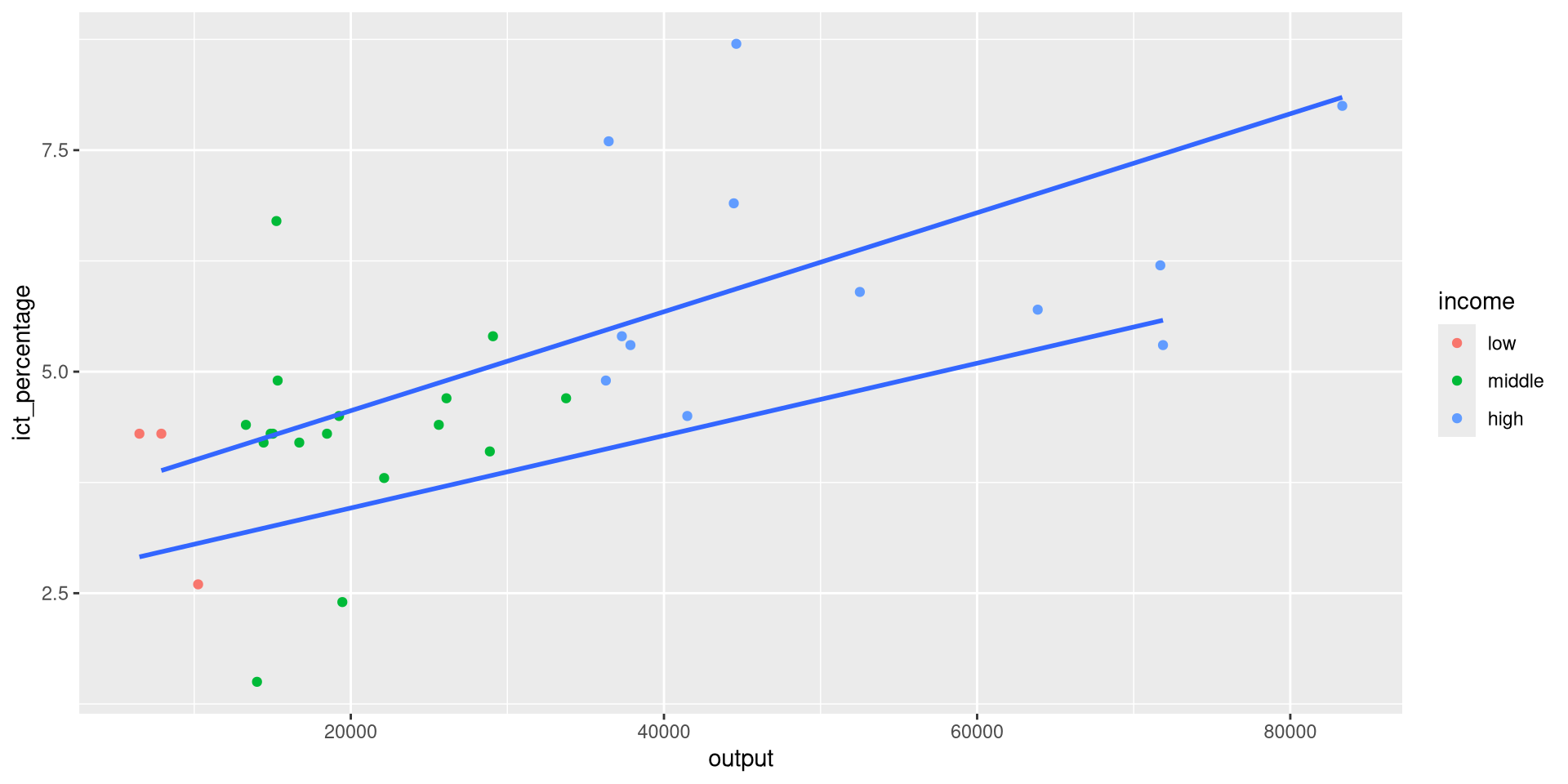
- We want to textually highlight regression lines per group.
- Suppose we want to add the country names at the end of each regression line.
- We can pick the maximum
outputvalue per group and use it as thexaesthetic ingeom_text().
Using geom_text(): Example 2
- We want to textually highlight regression lines per group.
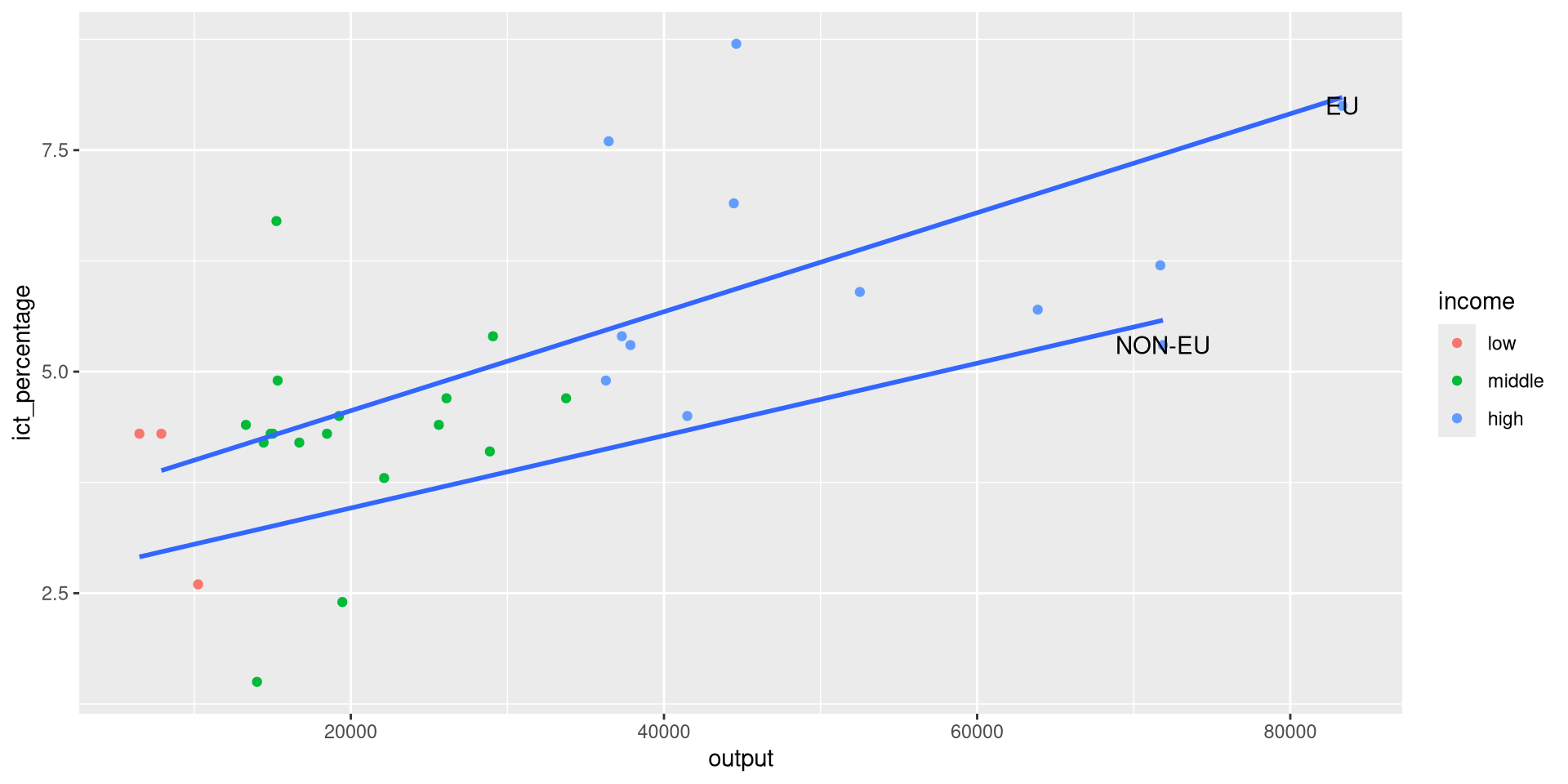
- We pass the aesthetics we want to use in the
mappingargument ofgeom_text().
Using geom_text(): Example 2
- We want to textually highlight regression lines per group.
ggplot(eu_ict, aes(output, ict_percentage)) +
geom_point(aes(color = income)) +
geom_smooth(
aes(group = EU), method = "lm", se = FALSE, formula = y ~ x
) +
geom_text(
data = eu_ict |>
dplyr::group_by(EU) |>
dplyr::slice_max(output, n = 1),
aes(output, ict_percentage, label = EU),
hjust = "left",
vjust = "bottom",
nudge_x = 1000
)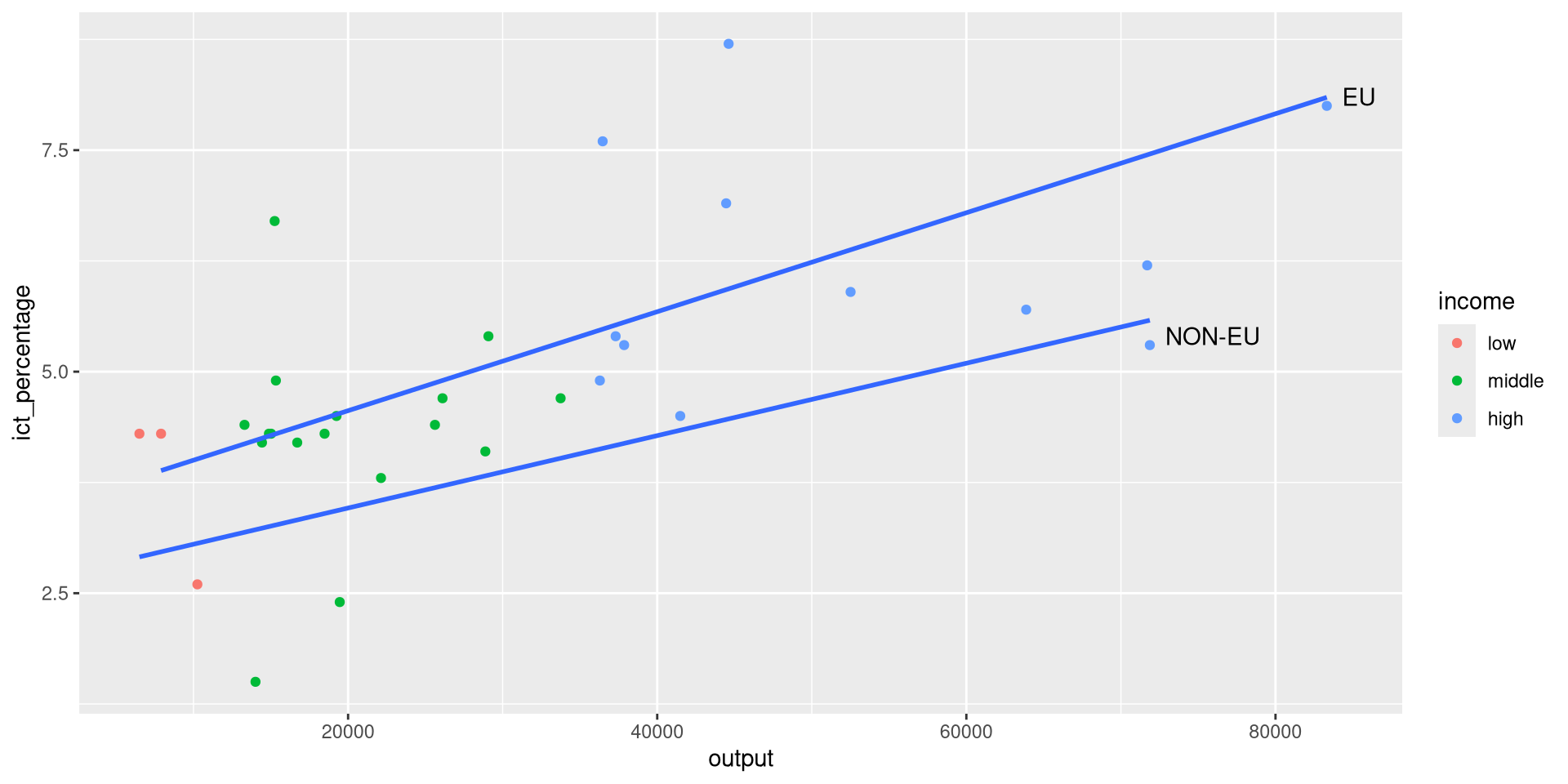
- And fine-tune the appearance of the text with
hjust,vjust, andnudge_x.
Using annotate() for text
- We want to add a label next to the richest EU country.

Using annotate() for text
- We want to add a label next to the richest EU country.

- And use the calculated
richestdata to pass more information toannotate().
Using annotate() for text
- We want to add a label next to the richest EU country.

- We can adjust the label’s text horizontal alignment.
Using annotate() for text
- We want to add a label next to the richest EU country.
- The
annotate()function does not havenudge_*arguments (why?).
- We can directly adjust the
xandypositions to move the label around.
Using annotate() for text
- We want to add a label next to the richest EU country.
Using annotate() for text

Using annotate() for segments

- We nudge the label of the richest country a bit more to the left.
Using annotate() for segments
richest <- eu_ict |>
dplyr::filter(EU == "EU") |>
dplyr::slice_max(output, n = 1)
ggplot(eu_ict, aes(output, ict_percentage)) +
geom_point(aes(color = income, shape = EU)) +
annotate(
geom = "label",
label = richest$geo,
x = richest$output - 8000,
y = richest$ict_percentage,
hjust = "right",
) +
annotate(
geom = "segment",
x = richest$output - 8000,
xend = richest$output - 500,
y = richest$ict_percentage,
yend = richest$ict_percentage
)
- This creates a segment connecting the two points, but not an arrowhead.
Using annotate() for segments
richest <- eu_ict |>
dplyr::filter(EU == "EU") |>
dplyr::slice_max(output, n = 1)
ggplot(eu_ict, aes(output, ict_percentage)) +
geom_point(aes(color = income, shape = EU)) +
annotate(
geom = "label",
label = richest$geo,
x = richest$output - 8000,
y = richest$ict_percentage,
hjust = "right",
) +
annotate(
geom = "segment",
x = richest$output - 8000,
xend = richest$output - 500,
y = richest$ict_percentage,
yend = richest$ict_percentage,
arrow = arrow(type = "closed", length = unit(0.3, "cm"))
)![]()
- We can add an arrowhead to the plot using the
arrowargument.
Using annotate() for segments
richest <- eu_ict |>
dplyr::filter(EU == "EU") |>
dplyr::slice_max(output, n = 1)
ggplot(eu_ict, aes(output, ict_percentage)) +
geom_point(aes(color = income, shape = EU)) +
annotate(
geom = "label",
label = richest$geo,
x = richest$output - 8000,
y = richest$ict_percentage,
hjust = "right",
) +
annotate(
geom = "segment",
x = richest$output - 8000,
xend = richest$output - 500,
y = richest$ict_percentage,
yend = richest$ict_percentage,
arrow = arrow(type = "closed", length = unit(0.3, "cm")),
color = "red"
)
- Finally, the color of the annotation can be adjusted with the
colorargument.
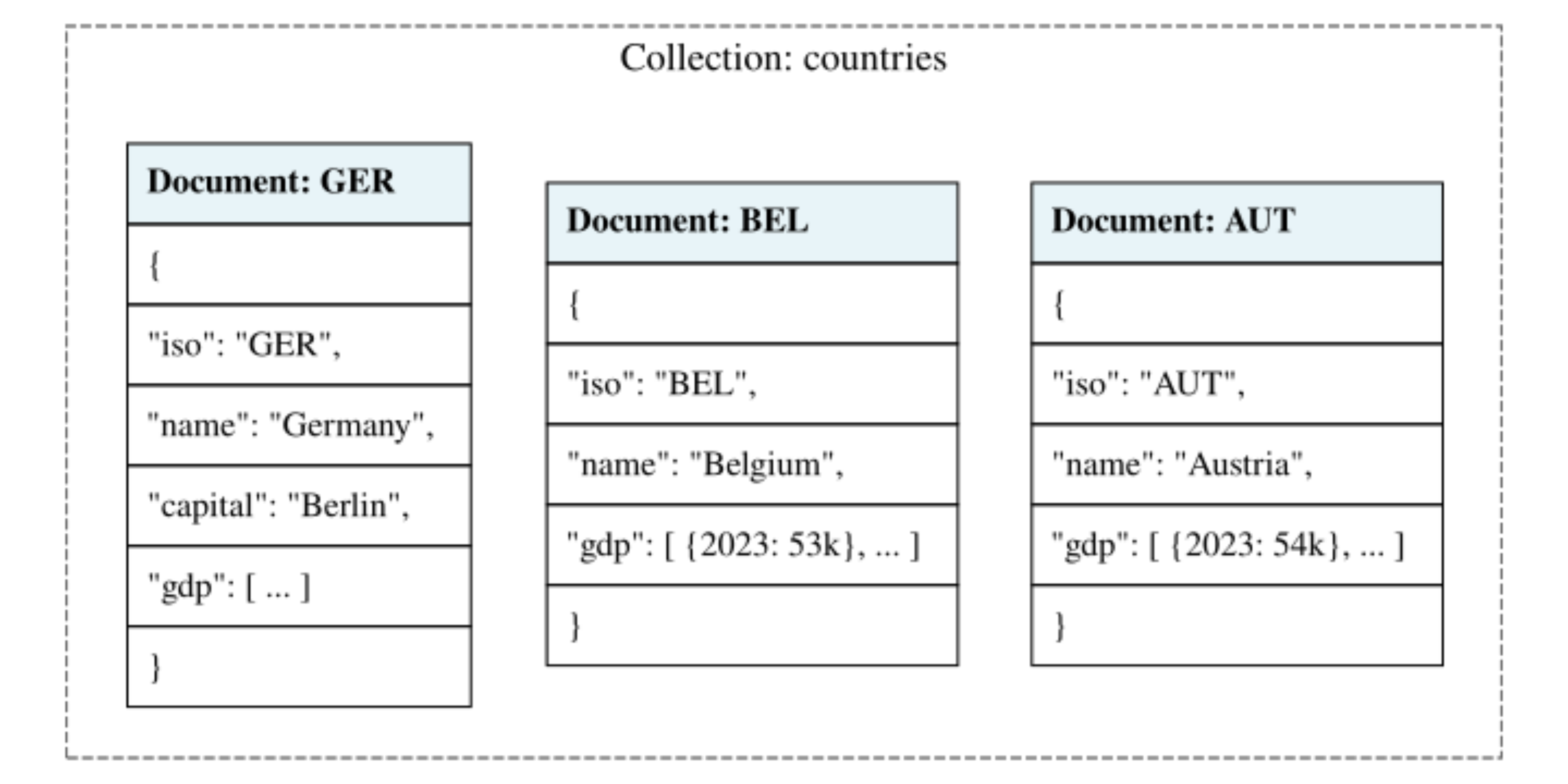
A relational example
- We can represent this data in a relational database with two tables:
country_metadataandgdp_data.
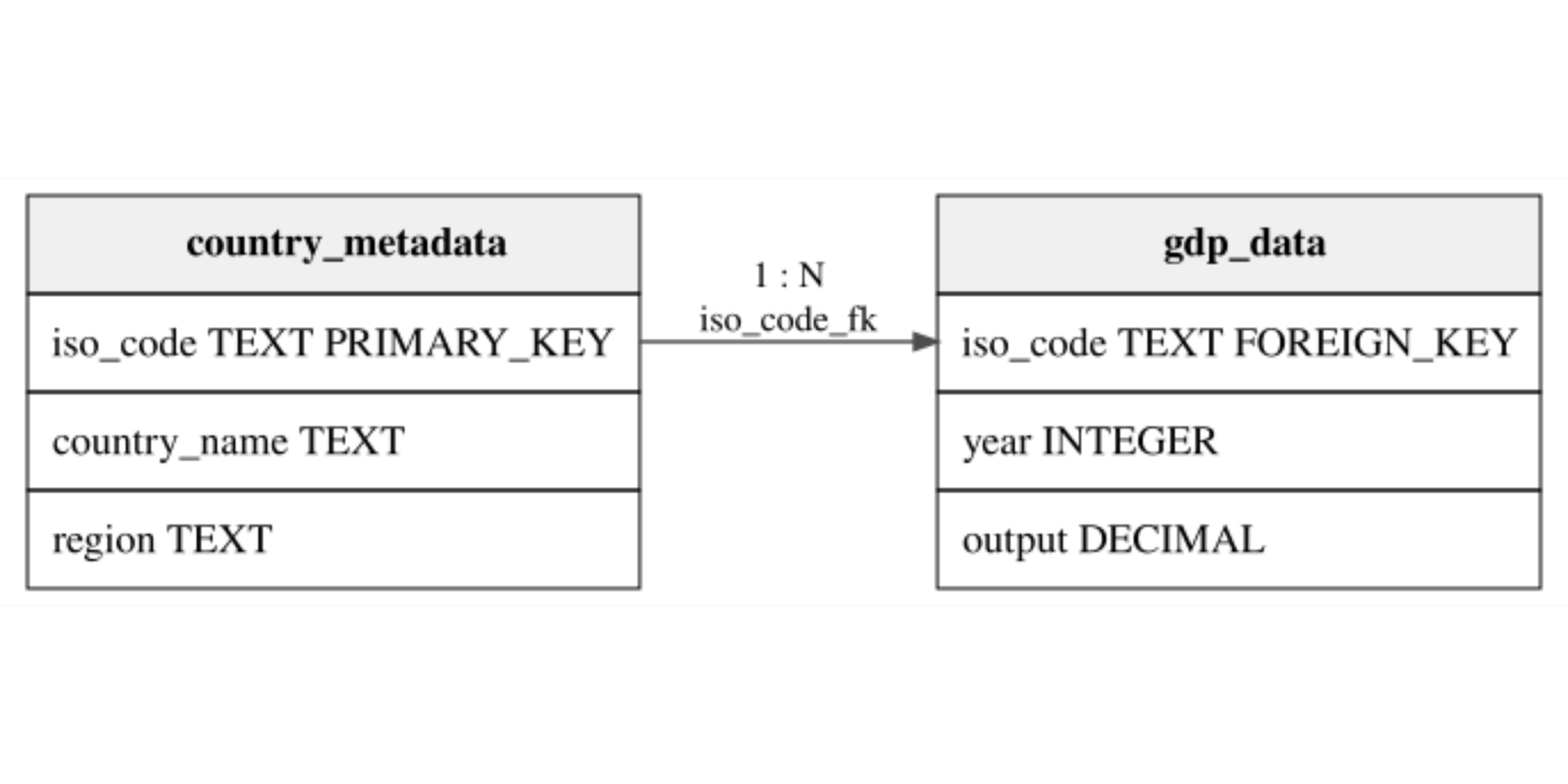
A relational example
- We can represent this data in a relational database with two tables:
country_metadataandgdp_data.
- The
country_metadatatable is the Dimension Table.- It contains static attributes that identify countries.
- The
gdp_datatable is the Fact Table.- It contains dynamic observations that can change over time.
A non-relational example