Working with Databases and Large Datasets
An introduction to managing and analyzing large datasets. Foundations of SQL and NoSQL databases. File-based databases. Mapping dplyr verbs to SQL queries.
1 Foundations of data storage
- In the previous topics, we worked with data loaded from files (e.g., CSV, Excel).
- This works fine for datasets of a few GB depending on your machine.
- What about larger datasets?
- In this topic, we discuss the fundamentals of data storage and retrieval when working with large datasets and emulate the workflow via an example using
DuckDB.
2 Basic background concepts
- We begin by discussing the following concepts.
- Data storage architectures:
- Distributed vs. centralized storage.
- The client-server pattern.
- Data structure:
- Relational (
SQL) vs. non-relational (NoSQL). - Row vs. columnar storage.
- Relational (
- Data Formats:
- Human-readable (
CSV,JSON,XML) vs. Binary (Parquet).
- Human-readable (
3 Storage architectures
The classic way of storing data uses the client-server architecture.
- The database server manages the data.
- Often, the main server has the ground-truth representation of the data.
- Replication servers are used for load balancing and backup purposes.
Storage architectures
The classic way of storing data uses the client-server architecture.
More recent storage architectures include distributed storage (e.g., Hadoop, Spark).
- Data is distributed across multiple machines.
- Allows for processing of large datasets that exceed the capacity of a single machine.
- Benefits scalability and fault tolerance, but introduces complexity in ensuring data consistency and managing transactions.
3.1 Client-server architecture
A (typically remote) machine runs a database server.
- A server is a program that continuously listens for requests.
- When a request arrives, the server processes it and sends back a response.
Client-server architecture
- A (typically remote) machine runs a database server.
A (typically local) machine runs a client program.
-  A client is a program that connects to the listening port of the server.
- It sends requests to the server and waits for responses.
Client-server architecture
- A (typically remote) machine runs a database server.
- A (typically local) machine runs a client program.
- Examples of client-server databases include PostgreSQL, MySQL, and Oracle Database.
4 Data structures
The traditional way of structuring databases is relational.
- Data is stored in tables (rows/columns).
- They follow a strict schema (predefined structure).
- Rows in tables can be identified by unique key values (primary key).
- Tables can have relationships with each other (e.g., foreign keys).
- Foreign keys are references to primary keys in other tables.
Data structures
The traditional way of structuring databases is relational.
The language of interacting with relational databases is
SQL(Structured Query Language).- Accessing and manipulating data has many analogies with the verbs we saw in
dplyr.
- Accessing and manipulating data has many analogies with the verbs we saw in
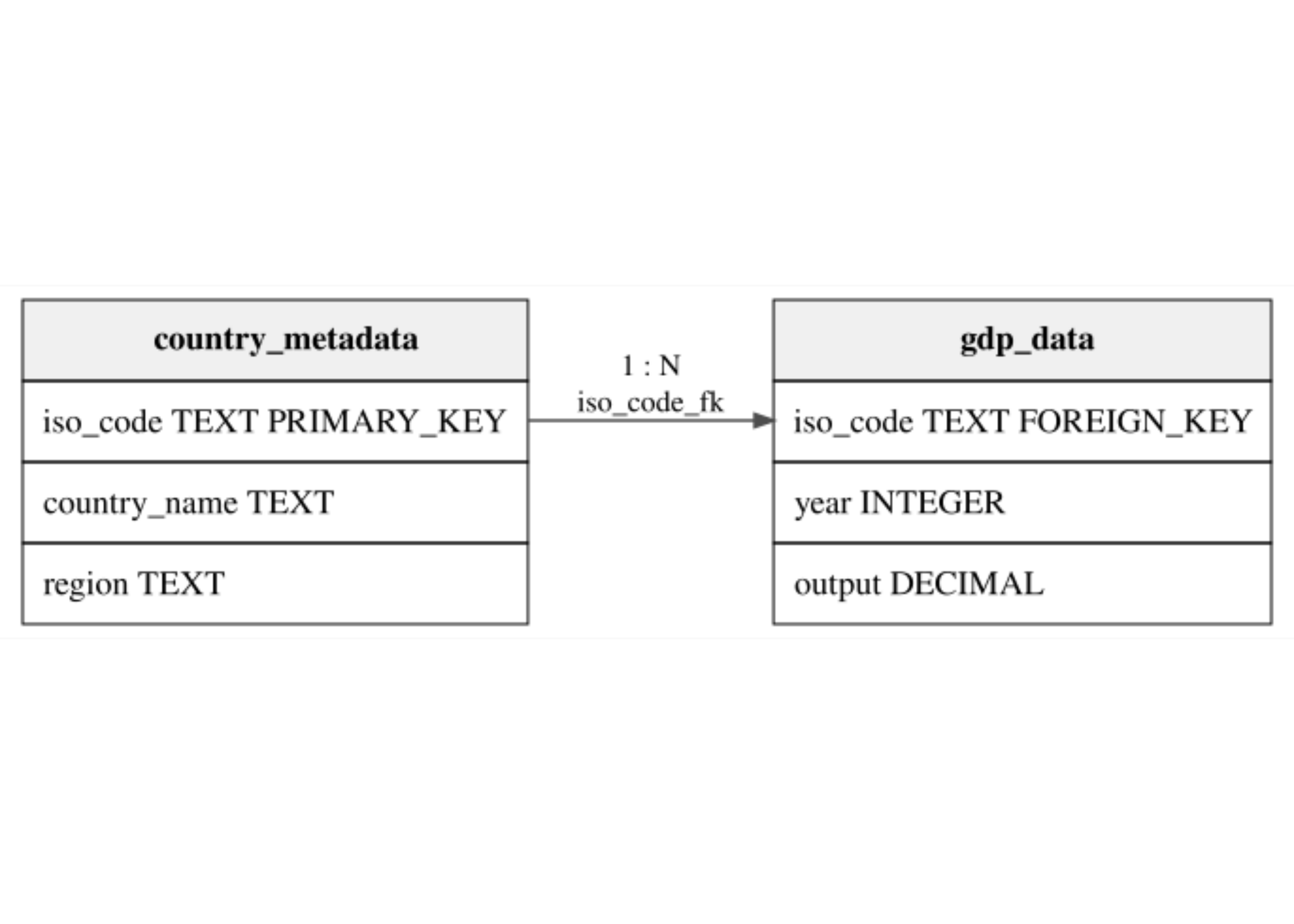
4.1 A relational example
- Suppose we have the following data
- Multiple country entries.
- Each country has a unique
iso_code. - Each country has multiple output values across years.
A relational example
- We can represent this data in a relational database with two tables:
country_metadataandgdp_data.
A relational example
- We can represent this data in a relational database with two tables:
country_metadataandgdp_data.
- The
country_metadatatable is the Dimension Table.- It contains static attributes that identify countries.
- The
gdp_datatable is the Fact Table.- It contains dynamic observations that can change over time.
4.2 Non-relational databases
Alternatives ways to structure data are often referred to as Non-relational.
- In modern lingo, these are often called
NoSQL(Not onlySQL) databases. - They are designed to handle large volumes of unstructured or semi-structured data.
- They are either schema-less or have a flexible schema.
- They often sacrifice some of the strict consistency guarantees of relational databases for improved scalability and flexibility.
- In modern lingo, these are often called
Non-relational databases
Alternatives ways to structure data are often referred to as Non-relational.
- Example: MongoDB (document store) and Neo4j (graph database).
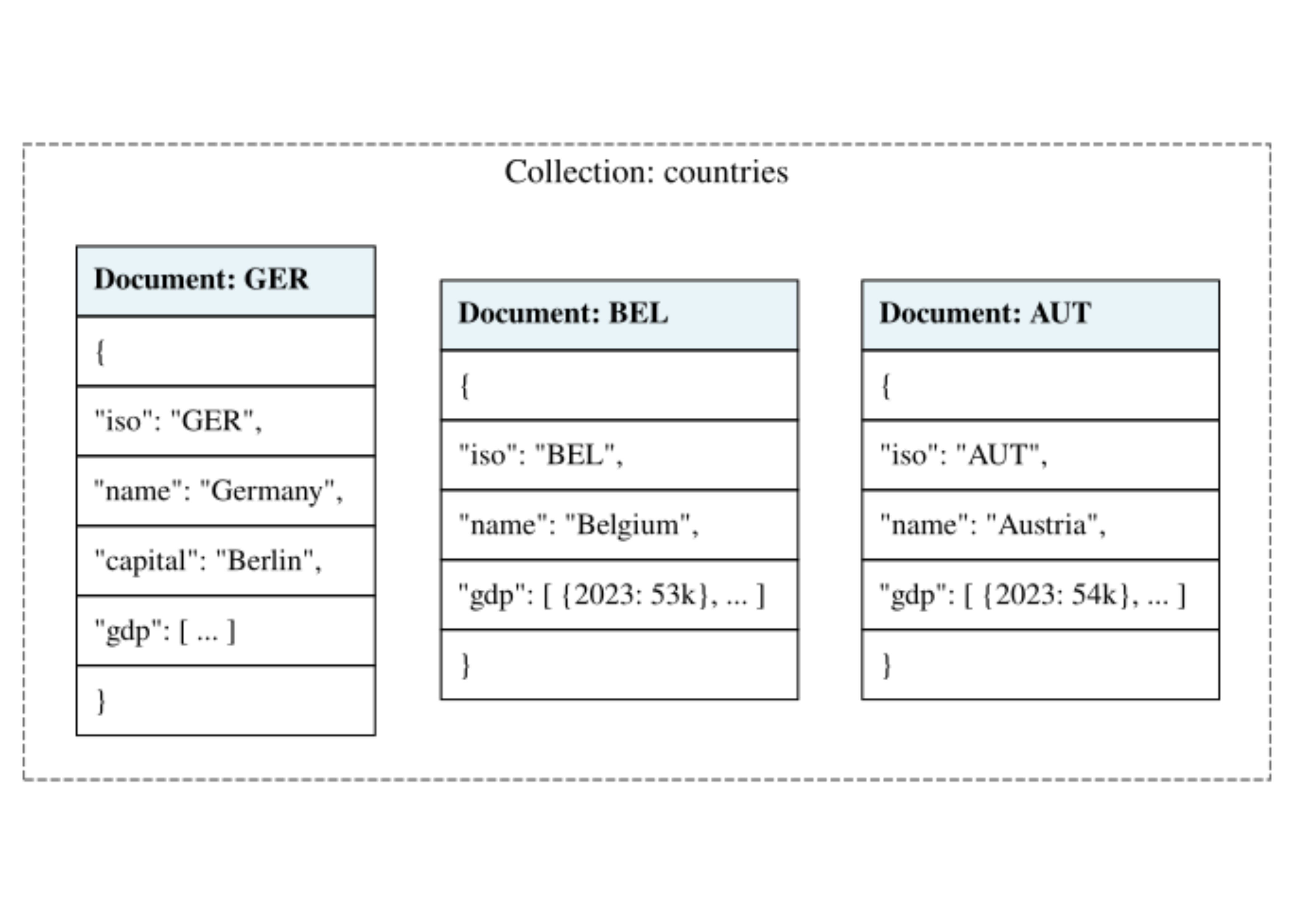
4.3 A non-relational example
- In a document store database, there are no tables.
- Data is stored in collections.
- A collection is a set of documents (usually
JSON). - Each document is self-contained: it includes the data and its description.
- Instead of linking a country (dimension) to its GDP (fact) via a key, we embed the GDP directly inside the country document.
A non-relational example
4.4 Programming digression: JSON data format
- The JSON (JavaScript Object Notation) is one the most common format for NoSQL databases and Web APIs.
- It is a text-based format that is easy for humans to read and machines to parse.
- Key characteristics:
- Key-Value pairs: Data is organized in “labels” and “values”.
- Hierarchical: It supports nested structures (lists within objects).
- Language Independent: Although it comes from JavaScript, almost every programming language (including R, see e.g.,
jsonlite) has libraries to work with JSON.
4.5 Programming digression: JSON Syntax
- JSON has two primary structures:
4.6 Programming digression: JSON Data Types
- JSON has four data types:
- String:
"Hello"(must use double quotes) - Number:
42or3.14 - Boolean:
trueorfalse - Null:
null - Object/Array: For nesting.
4.7 Programming digression: Self-describing hierarchies
- We can represent complex hierarchies in a single file:
4.8 Programming digression: JSON vs. CSV
| Feature | CSV | JSON |
|---|---|---|
| Structure | Flat (Table) | Nested (Tree) |
| Metadata | Header only | Keys in every record |
| Readability | Hard for nested data, easy for tabular | Easy for nested data, harder for tabular |
| File size | Smaller | Larger (labels repeat) |
4.9 SQL vs. NoSQL: Which data structure to use?
- There is no best data structure.
- Perhaps, the most crucial point is whether data consistency is important.
- Are there multiple clients that need to read/write the same data?
- Do they need to see the same exact data at every point in time?
- If yes, then a relational database is likely a good choice.
SQL vs. NoSQL: Which data structure to use?
- There is no best data structure.
- In data science, we often only use read operations on data that is not changing (e.g., historical data).
- We modify or enrich data locally, but typically do not need to share back (write) our changes to the data source.
- Speed and simplicity of access are more important than strict consistency guarantees.
- For these reasons, non-relational databases are often a good choice.
4.10 Row vs. Column Storage
- Suppose that we want to store the following tabular dataset (e.g., a data frame) persistently on disk.
- There are two main ways to store this data:
- Row-based: Store the data row by row, with conservative elements of the same row stored together.
- Columnar: Store the data column by column, with all elements of the same column stored together.
Row vs. Column Storage
- Suppose that we want to store the following tabular dataset (e.g., a data frame) persistently on disk.
- In programming languages, similar concepts for storing arrays are called row-major and column-major order.
- By default,
RandMatlabuse column-major order, whilePythonandCuse row-major order.
Row vs. Column Storage
- Row-based (CSV, most relational databases):
- Optimized for adding or updating individual rows.
- However, to read one column, one must scan the entire file.
- Columnar (Parquet, DuckDB):
- Optimized for analytical queries.
- Reads only the columns you need, however consistently modifying data becomes more complex.
5 Connecting R to Databases
- We want to connect
Rto a database.
- We use a common interface called DBI (DataBase Interface).
Connecting R to Databases
- We want to connect
Rto a database.
- The
DBIPackage gives unified framework for communicating with different database management systems (DBMS).
- It separates the connection logic from the data manipulation logic.
- In this way we use the same R commands to talk to PostgreSQL, MySQL, SQLite, or DuckDB.
Connecting R to Databases
- We want to connect
Rto a database.
- Each database needs a specific “driver” (e.g.,
RPostgres,RSQLite,duckdb).
- The driver translates
DBIcommands into the specific “dialect” of that database.
Connecting R to Databases
- We want to connect
Rto a database. - Each database needs a specific “driver” (e.g.,
RPostgres,RSQLite,duckdb).
- Postgres:
Postgres()from theRPostgrespackage.
- MySQL:
MySQL()from theRMySQLpackage. - SQLite:
SQLite()from theRSQLitepackage. - DuckDB:
duckdb()from theduckdbpackage.
5.1 The DBI Workflow
- The standard workflow involves three main steps:
- Connect: Establish a connection between
Rand the database usingdbConnect(). - Interact: Send queries or commands using
dbGetQuery()ordbExecute(). - Disconnect: Close the connection with
dbDisconnect()to free up resources.
5.2 Introduction to DuckDB
- For this topic, we focus on DuckDB.
- DuckDB is an “in-process” SQL Online Analytical Processing (OLAP) DBMS.
Introduction to DuckDB
- In-process: No server to install. The database runs in the computer’s memory.
- OLAP: Optimized for analytical queries (aggregations, selections, transformations) rather than updates.
- Columnar: Stores data by column.
- Portable: Can run on a local file or entirely in one’s computer RAM.
5.3 Connecting to DuckDB
- Using the
duckdbpackage withDBI:
Persistent Connection
- Data is saved to a file on disk.
- Persists after the R session ends.
5.4 Working with DuckDB: Basic Operations
- Once connected, one gets integration with
R’s data structures.
Working with DuckDB: Basic Operations
- Once connected, one gets integration with
R’s data structures.
Listing Tables in the database:
Working with DuckDB: Basic Operations
- Once connected, one gets integration with
R’s data structures.
Reading Data to
Rdata frames using SQL queries:
5.5 Working with DuckDB: Querying External Files
- A nice
DuckDBfeature is its ability to query external files without importing them.
It can directly scan CSV, JSON, and Parquet files.
              DATAFLOW         LAST UPDATE   freq
1 ESTAT:SDG_08_10(1.0) 2020-12-24 11:00:00 Annual
2 ESTAT:SDG_08_10(1.0) 2020-12-24 11:00:00 Annual
3 ESTAT:SDG_08_10(1.0) 2020-12-24 11:00:00 Annual
                                          unit
1 Chain linked volumes (2010), euro per capita
2 Chain linked volumes (2010), euro per capita
3 Chain linked volumes (2010), euro per capita
                                  na_item     geo TIME_PERIOD OBS_VALUE
1 Gross domestic product at market prices Albania        2000      1700
2 Gross domestic product at market prices Albania        2001      1850
3 Gross domestic product at market prices Albania        2002      1940
  OBS_FLAG
1     <NA>
2     <NA>
3     <NA>
6 The universality of data transformations
- The logic of data transformations we have seen in
dplyris universal and applies to databases as well.
- The transformations are supported in SQL and, as a result, also in
DuckDB. - We demonstrate this by showing the SQL equivalent of the
dplyrcode we have seen in previous topics.
6.1 Selecting columns
6.2 Selecting columns with distinct values
6.3 Selecting and renaming columns
6.4 Mutating values of columns
6.5 Filtering observations
6.6 Arranging observations
6.7 Relocating columns
6.8 Verification
- We have focused on the syntax of SQL queries so far. Can we verify that the results between the
dplyrandSQLcode are the same? - Let us compare the
selectresults.
Verification
- Let us compare the
selectresults.
[1] "Attributes: < Component \"class\": Lengths (3, 1) differ (string compare on first 1) >"
[2] "Attributes: < Component \"class\": 1 string mismatch >"
[3] "Component \"unit\": 924 string mismatches"
[4] "Component \"geo\": 1793 string mismatches"
[5] "Component \"TIME_PERIOD\": Mean relative difference: 0.004086815"
[6] "Component \"OBS_VALUE\": Mean relative difference: 1.372438"
[7] "Component \"OBS_FLAG\": 'is.NA' value mismatch: 1721 in current 1721 in target" - Why do we get so many mismatches?
Verification
- Let us compare the
selectresults.
[1] "Attributes: < Component \"class\": Lengths (3, 1) differ (string compare on first 1) >"
[2] "Attributes: < Component \"class\": 1 string mismatch >" - What do these differences mean?
Verification
- Let us compare the
selectresults.
dfl <- sdg |>
  select(unit, geo, TIME_PERIOD, OBS_VALUE, OBS_FLAG) |>
  arrange(unit, geo, TIME_PERIOD, OBS_VALUE, OBS_FLAG)
dfr <- dbGetQuery(con, '
  SELECT DISTINCT
    unit, geo, "TIME_PERIOD", "OBS_VALUE", "OBS_FLAG"
  FROM sdg
  ORDER BY unit, geo, TIME_PERIOD, OBS_VALUE, OBS_FLAG;
') |>
  as_tibble()
all.equal(dfl, dfr)
[1] TRUE7 Data persistence and portability
- An advantage of using a databases is portability.
- Language Agnostic Access: One can write data in
Rand read it inPython(or any other language). - We have already written the
sdgdata frame to aDuckDBdatabase. - We will access it and select data in
Python.
Data persistence and portability
- An advantage of using a databases is portability.
- First we disconnect from
R(Why?)
Data persistence and portability
- An advantage of using a databases is portability.
- We connect to the same database file in
Python.
Data persistence and portability
- An advantage of using a databases is portability.
- And retrieve the data using the same
SQLquery as inR.
               DATAFLOW         LAST UPDATE    freq  ... TIME_PERIOD OBS_VALUE OBS_FLAG
0  ESTAT:SDG_08_10(1.0) 2024-12-20 11:00:00  Annual  ...        2000    1700.0     None
1  ESTAT:SDG_08_10(1.0) 2024-12-20 11:00:00  Annual  ...        2001    1850.0     None
2  ESTAT:SDG_08_10(1.0) 2024-12-20 11:00:00  Annual  ...        2002    1940.0     None
3  ESTAT:SDG_08_10(1.0) 2024-12-20 11:00:00  Annual  ...        2003    2060.0     None
4  ESTAT:SDG_08_10(1.0) 2024-12-20 11:00:00  Annual  ...        2004    2180.0     None

[5 rows x 9 columns]