Dynamic Competition

Context

• Competition in real markets is not a static phenomenon. Firms can change their choices from date to date and adapt their strategies based on past events and the reactions of competitive firms.

• In such fluid settings, some firms take the initiative and set the pace of competition in the market. Other firms follow.
  • Do firms benefit from assuming a market leader role?
  • How does the sequence of moves affect the market power?
  • Why does market entry influence the behavior of incumbent firms?

Course Structure Overview

Lecture Structure and Learning Objectives

Structure

• The Model T (Case Study)
• The Stackelberg model
• Sequential Competition in Prices
• The Role of Market Entry in Competition
• Current Field Developments

Learning Objectives

• Describe the impact of move order on market power under quantity competition.
• Describe the impact of move order on market power under price competition.
• Highlight the welfare effects of leadership under various competition means.
• Illustrate the effect of free entry in dynamic competition.
• Illustrate the importance of credibility in entry deterrence.

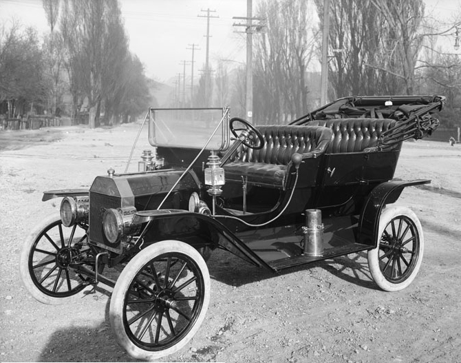
The Model T

People can have the model T in any color—so long as it’s black.

Henry Ford

Ford vs General Motors

• Ford and General Motors are two of the largest automobile companies worldwide.
• They were both founded in the beginning of the \(20^{\text{th}}\) century.
• Since then, they have been competing for the lead in the US automobile market.

Third Time is a Charm

Fordism

Game On

The Market Leader

• Model T’s production innovations made Ford the leading car company from about 1910 to 1925.

• The reluctance of Ford to keep introducing innovations and the absence of flexibility changed the situation.
• In 1925, GM surpassed Ford in total revenue and kept ahead until 1986.
• Eventually in 1927, Ford shutdown for 6 months to update its production lines for Model A.
• GM also surpassed Ford in total sales during this period.

Leader-follower Competition in Quantities

• The Stackelberg model of oligopoly describes a market structure with two or more firms such that
  • the market does not suffer from any other market failure (imperfect information, externalities, etc),
  • no other firms can enter the market,
  • firms sell a homogeneous product,
  • firms try to maximize their profits,
  • consumers are price takers, firms choose the quantities that they produce, the leader chooses first, and the follower(s) choose afterward, and
  • consumers try to maximize their utility.

Residual Demand

• The leader chooses the quantity it produces first.
• Thus, the follower does not face the entire market demand but only the demand remaining after the leader’s choice.
• The difference between the market demand and the aggregated supplied quantities of all competitive firms is a firm’s residual demand.

The Follower’s Problem

• We solve the problem with backward induction.
• The follower claims the residual demand.
• For any given quantity \(q_{1}\) produced by the leader, the follower’s problem is

\[\max_{q_{2}} \left\{ p(q_{1} + q_{2})q_{2} - c_{2}(q_{2}) \right\}.\]

• Interior optimal solutions require

\[p’(q_{1} + q_{2})q_{2} + p(q_{1} + q_{2}) = c_{2}’(q_{2}).\]

• From this condition, we obtain (solving for \(q_{2}\)) the best response of the follower, say

\[q_{2} = b_{2}(q_{1}).\]

The Leader’s Problem

• The leader anticipates the best response of the follower and solves

\[\max_{q_{1}} \left\{ p(q_{1} + b_{2}(q_{1}))q_{1} - c_{1}(q_{1}) \right\}.\]

• Its optimality condition is given by

\[p’(q_{1} + b_{2}(q_{1})) \left(1 + b_{2}’(q_{1})\right) q_{1} + p(q_{1} + b_{2}(q_{1})) = c_{1}’(q_{1}).\]

An Analytic Example

• Suppose that the demand and cost functions are given by

  \begin{align*} p(q) &= p_{0} + p_{1} q, \\ c_{1}(q_{1}) &= c q_{1}, \\ c_{2}(q_{2}) &= c q_{2}. \end{align*}

The Follower’s Problem

• The follower’s necessary condition becomes

\[p_{1}q_{2} + p_{0} + p_{1}(q_{1} + q_{2}) = c.\]

• Then, the best response of the follower is

\[b_{2}(q_{1}) = \frac{c - p_{0} - p_{1}q_{1}}{2 p_{1}}.\]

The Leader’s Problem

• The leader solves

\[\max_{q_{1}} \left\{ p\left(q_{1} + \frac{c - p_{0} - p_{1}q_{1}}{2 p_{1}}\right)q_{1} - c(q_{1}) \right\}.\]

• Its optimality condition is given by

\[\frac{p_{1}}{2}q_{1} + p_{0} + \frac{c - p_{0}}{2} + \frac{p_{1}}{2}q_{1} = c.\]

• Therefore, the leader produces

\[q_{1}^{\ast} = \frac{c - p_{0}}{2 p_{1}}.\]

Market Quantity and Price

• Given the leader’s quantity, the follower produces

\[q_{2}^{\ast} = b_{2}(q_{1}^{\ast}) = \frac{c - p_{0}}{2 p_{1}} - \frac{1}{2}\frac{c - p_{0}}{2 p_{1}} = \frac{c - p_{0}}{4 p_{1}}.\]

• The market quantity is

\[q^{\ast} = q_{1}^{\ast} + q_{2}^{\ast} = 3\frac{c - p_{0}}{4 p_{1}}.\]

• The market price is

\[p(q^{\ast}) = p_{0} + p_{1} q^{\ast} = \frac{p_{0} + 3 c}{4}.\]

Profits

• The follower makes profit

\[\pi_{2} = \left(p(q^{\ast}) - c\right) q_{2}^{\ast} = - \frac{\left(p_{0} - c\right)^{2}}{16p_{1}}.\]

• The leader’s profit is

\[\pi_{1} = \left(p(q^{\ast}) - c\right) q_{1}^{\ast} = - \frac{\left(p_{0} - c\right)^{2}}{8p_{1}}.\]

First Move Advantage

• The firms’ profits in the Cournot model with symmetric costs are

\[\pi_{c} = - \frac{\left(p_{0} - c\right)^{2}}{9p_{1}}.\]

• Compared to the firms’ profits in the Cournot model, we have

\[\pi_{1} > \pi_{c} > \pi_{2}.\]

• The leader makes more profit compared to Cournot competition, while the follower makes less profit.
• However, aggregate profits in the market are less compared to Cournot, i.e.,

\[\pi_{1} + \pi_{2} < 2 \pi_{c}.\]

Leader-Follower Competition in Prices

• Consider a variation of the Stackelberg game in which firms are price setters.

• This is the sequential version of the Bertrand model.

• There are two firms \((i, j \in \{1,2\})\) with marginal cost equal to \(c\).

• Firm \(1\) is the leader (moves first), and firm \(2\) is the follower (moves second).

• The demand for firm \(i\) is

  \begin{align*} d_{i}(p_{i}, p_{j}) = \left\{\begin{aligned} &10 - \frac{1}{2}p_{i} & p_{i} < p_{j} \\ &5 - \frac{1}{4}p_{i} & p_{i}=p_{j} \\ &0 & p_{i} > p_{j} \end{aligned}\right.. \end{align*}

• The firm with the lowest price gets all the demand.

• If prices are equal, demand is equally split.

Non Equilibrium Prices

• Suppose that firm \(1\) sets a price \(p_{1}\) that is greater than the marginal cost of firm \(2\) (i.e., \(c\)).
• Firm \(2\) can undercut by a small amount and grab all the market. For instance, set price \(p_{2} = \frac{c + p_{1}}{2}\).
• Thus, firm \(1\) can only set a price equal to firm \(2\)’s marginal cost.

Equilibrium

• The only possible equilibrium is both firms to set a price equal to the (common) marginal cost.
• Firms do not have any incentive to deviate.
• Setting lower prices leads to losses.
• Setting higher prices leads to zero profits.
• The order with which firms move does not affect the market outcome.

A Game of Market Entry

• Consider a market with one firm already operating and a potential entrant.
• The entrant decides whether to enter the market.
• The incumbent decides whether to follow aggressive or complying competition behavior.

Entry Deterrence with Credible Threat

• \(SPE = \left\{ \left(Stay\ out, Fight \right) \right\}\)

Entry with Non-Credible Threat

• \(SPE = \left\{ \left(Enter, Don’t\ fight \right) \right\}\)

Quantity Competition with Costly Entry

• We extend the Cournot duopoly model by allowing firms to choose whether they enter the market.
• Firms enter the market when they can make profits.
• Firms incur a fixed cost \(\bar c\) upon entry.

Market and Dynamics

• There is an infinite number of potential entrants.
• The market’s inverse demand is

\[p(q) = p_{0} + p_{1}q \quad(p_{0}>0,\ p_{1}<0).\]

• All firms have costs

\[c(q) = c_{1}q \quad(c_{1}>0).\]

• The firms that enter the market choose their quantities at the second date simultaneously.
• At the first date, the entrants decide how many of them enter the market.

Unregulated Entry and Exit

• When \(n\) firms enter the market, each firm makes profit

\[\pi_{i}(n) = -\frac{(c_{1} - p_{0})^{2}}{(n + 1)^{2} p_{1}} - \bar c.\]

• In equilibrium

\[\pi_{i}(n^{e}) = 0 \iff n^{e} = \frac{p_{0} - c_{1}}{\sqrt{- \bar c p_{1}}} - 1.\]

The Social Welfare

• The social welfare is calculated by

\[W(n) = \int_{0}^{n} p(s q(s)) \left(q(s) + sq’(s)\right) \mathrm{d} s - n c(q(n)) - n \bar c.\]

The First Best Solution

• Aggregate profit is maximized when

\[p(n q(n))\left(q(n) + n q’(n)\right) - c(q(n)) - n c’(q(n))q’(n) = \bar c .\]

• This implies that

\[n^{*} = \sqrt[3]{-\frac{(p_{0} - c_{1})^{2}}{p_{1} \bar c}} - 1 .\]

• Comparing with the unregulated entry equilibrium, we have

\[ n^{*} < n^{e} .\]

• With quantity competition, unregulated entry results in excessive entry of firms.

Current Field Developments

• Market dynamics and entry constitute important components of competition policy.
• Mergers and acquisitions are dynamic phenomena modifying the number of firms in the market and their market power.
• Merger cases are central from both an economic and competition law perspective.
• In the US and EU, antitrust laws aim to reduce or avoid excessive market concentration.
• Dynamic market models are commonly used to assess mergers and their impact on market power in court cases.

Comprehensive Summary

• The sequence with which firms act in a market can influence market power.
  • If firms compete in quantities, then the leader has a first move advantage.
  • If firms compete in prices, then the sequence of moves is irrelevant.
• Competition forces do not concern only firms who already entered in a market.
• Incumbent firms strategically interact with potential competitors looking to enter the market.
• Free entry is a characteristic of market competition that can reduce firms’ profits and result to low prices.
• On some occasions (e.g. entry costs), excessive entry can result to economic inefficiencies.

Further Reading

• Belleflamme & Peitz, 2010, secs. 4.1, 4.2.1-3
• Varian, 2010, secs. 28.2, 29.8

Exercises

Group A

1. Consider an endogenous timing game in which firms simultaneously choose whether to play \(Early\) or to play \(Late\) . If both firms make the same choice, then they compete as in Bertrand competition. If the firms make different choices, then they compete as in the Stackelberg model (sequential competition in quantities), where the leader is the firm that chose \(Early\) and the follower is the firm that chose \(Late\). Suppose that firms have cost functions to \(c(q)=q\), and market demand is given by \(p(q) = 5 - q\).

   1. Calculate the profits of the firms under the different means of competition.
   2. Draw the extensive form of the game.
   3. Calculate all the Nash Equilibria.
   1. If the firms compete simultaneously using prices, they set \(p_{1} = p_{2} = 1\) and make zero profits. If they compete sequentially using quantities, the follower makes profit \[\pi_{f} = \frac{(5-1)^{2}}{16} = 1,\] and the leader makes profit \[\pi_{l} = \frac{(5-1)^{2}}{8} = 2.\]
   2. The extensive form of the game is
   3. There are two pure strategy Nash equilibria, namely \[\left\{\left\{Early, Late\right\}, \left\{Late, Early\right\}\right\},\] and a mixed strategy equilibrium in which each firm chooses \(Early\) with probability \(p=\frac{2}{3}\).

Group B

1. Consider the quantity competition with costly entry game. Suppose that firms face market demand \(p(q) = p_{0} + p_{1}q\), have symmetric production costs \(c(q)=c_{1}q\), and entry costs \(\bar c\), where \(p_{0}, c_{1} > 0\) and \(p_{1}<0\). The social welfare as a function of the number of firms is given by \[W(n) = \int_{0}^{n} p(s q(s)) \left(q(s) + sq’(s)\right) \mathrm{d} s - n c(q(n)) - n \bar c .\] Calculate the Pareto optimal number of entrants in the market.

   1. By Fermat’s theorem, the welfare is maximized when \(W’(n) = 0\). Using the fundamental theorem of calculus, we get \[p(n q(n))\left(q(n) + n q’(n)\right) - c(q(n)) - n c’(q(n))q’(n) = \bar c.\] The optimal quantity produced by each firm when \(n\) firms enter the market is \[q(n) = -\frac{p_{0} - c_{1}}{(n + 1) p_{1}},\] hence, one calculates \[\frac{q’(n)}{q(n)} = \frac{1}{n + 1}.\] We will use the last expression to simplify the first order condition. Rearranging the necessary condition and using the linearity of costs gives

      \begin{align*} \bar c &= p(n q(n))\left(q(n) + n q’(n)\right) - c(q(n)) - n c’(q(n))q’(n) \\ &= p(n q(n))q(n) - c(q(n)) + n \left(p(n q(n)) - c’(q(n))\right)q’(n) \\ &= \pi(n) + n \left(p(n q(n))q(n) - c(q(n))\right) \frac{q’(n)}{q(n)} \\ &= \pi(n) \left(1 + n \frac{q’(n)}{q(n)}\right) \\ &= \pi(n) \left(1 - n \frac{1}{n + 1}\right) \\ &= \pi(n) \left(\frac{1}{n + 1}\right). \end{align*}

      The profit of each firm when \(n\) firms enter the market is \[\pi(n) = -\frac{(p_{0} - c_{1})^{2}}{(n + 1)^{2} p_{1}},\] so, we get

      \begin{align*} \bar c &= -\frac{(p_{0} - c_{1})^{2}}{(n + 1)^{3} p_{1}}. \end{align*}

      Therefore, the socially optimal number of firms is given by

      \begin{align*} n &= \sqrt[3]{-\frac{(p_{0} - c_{1})^{2}}{p_{1} \bar c}} - 1. \end{align*}

References

References

Topic's Concepts

• residual demand
• stackelberg