Strategic Interactions in Markets
Table of Contents
- 1. Markets, Games, and Competition
- 2. Simultaneous Games
- 2.1. Context
- 2.2. Course Structure Overview
- 2.3. Lecture Structure and Learning Objectives
- 2.4. Street Fighter Mechanics
- 2.5. Social Dilemmas
- 2.6. Social Interactions
- 2.7. Representations of Games
- 2.8. Best Responses
- 2.9. Nash Equilibria
- 2.10. The Grappler Game
- 2.11. Mixed strategies
- 2.12. The Grappler Game's Equilibrium
- 2.13. Rock Paper Scissors
- 2.14. Current Field Developments
- 2.15. Concise Summary
- 2.16. Further Reading
- 2.17. Mathematical Details
- 2.18. Exercises
- 3. Simultaneous Competition
- 3.1. Context
- 3.2. Course Structure Overview
- 3.3. Lecture Structure and Learning Objectives
- 3.4. Microsoft's Pricing Strategies
- 3.5. Competition and Cooperation
- 3.6. Competition in Quantities
- 3.7. Quantity Competition with two Firms
- 3.8. Quantity Competition with More than two Firms
- 3.9. A Cournot Competition Exercise
- 3.10. Competition in Prices
- 3.11. A Bertrand Competition Exercise
- 3.12. Spatial Competition
- 3.13. Current Field Developments
- 3.14. Concise Summary
- 3.15. Further Reading
- 3.16. Mathematical Details
- 3.17. Exercises
- 4. Dynamic Games
- 5. Dynamic Competition
- 5.1. Context
- 5.2. Course Structure Overview
- 5.3. Lecture Structure and Learning Objectives
- 5.4. The Model T
- 5.5. Leader-follower Competition in Quantities
- 5.6. Leader-Follower Competition in Prices
- 5.7. A Game of Market Entry
- 5.8. Quantity Competition with Costly Entry
- 5.9. Current Field Developments
- 5.10. Concise Summary
- 5.11. Further Reading
- 5.12. Mathematical Details
- 5.13. Exercises
- 6. Collusion and Market Power
- 6.1. Context
- 6.2. Course Structure Overview
- 6.3. Lecture Structure and Learning Objectives
- 6.4. Our Customers are Our Enemies
- 6.5. Tacit Collusion
- 6.6. Tacit Collusion in Quantity Competition
- 6.7. Tacit Collusion in Price Competition
- 6.8. Market Power
- 6.9. Current Field Developments
- 6.10. Concise Summary
- 6.11. Further Reading
- 6.12. Mathematical Details
- 6.13. Exercises
- References
1. Markets, Games, and Competition
1.1. Context
- The majority of economic transactions take place through markets. Markets have a myriad of different structures. They are central in organizing production and allocating surpluses between participants. On some occasions, market participants cannot affect the outcome.
- However, on other occasions, market participants can follow complicated strategies to affect production allocation in their favor.
- What kind of strategies do market participants employ?
- How do the strategies of different participants interact?
- Do their strategies affect market efficiency besides allocation?
1.2. Course Structure Overview

1.3. Lecture Structure and Learning Objectives
Structure
- Jonathan Lebed (Case Study)
- Markets, Strategies, and Game Theory
- Basic Foundations
- Current Field Developments
Learning Objectives
- Explain what a market is from an economic perspective.
- Illustrate why participants' interactions are central in determining outcomes and allocations.
- Review the fundamental market structures (monopoly and perfect competition).
- Give a high-level overview of the alternative market structures and competition strategies.
1.4. Jonathan Lebed
- Lebed is a former stock market trader.
- He was raised in New Jersey, US.
- He was prosecuted by the US Securities and Exchange Commission (SEC) for stock manipulation.
- Lebed reached an out-of-court settlement with SEC in 2000; He was 15 years old.
1.4.1. The SEC Prosecution
- Lebed is the first minor ever prosecuted for stock-market fraud.
- Lebed tools were
- an America Online (AOL) internet connection,
- an E*trade account, and
- four email accounts in Yahoo Finance Message Boards.
- The SEC accused him of making his money through a pump and dump strategy.
1.4.2. Timeline
 Lewis (2001)
- Shortly after his \(11\text{-th}\) birthday Jonathan opened an account with America Online.
- He started building a website about pro-wrestling.
- At the age of 12, he invested \($8000\) (via his father) in the stock market, taken from a bond his parents gave him at birth.
- He started building an amateur investor website www[dot]stock-dogs[dot]com"
- At 14, the SEC charged him with civil fraud.
- His mother closed his trading account.
- His father opened another account for him!
1.4.3. The Settlement
- Lebed forfeited \($285000\) in profit and interest he had made on \(11\) trades.
- He has never admitted any wrongdoing.
- He kept close to \($500000\) in profit.
1.4.4. Everybody is Manipulating the Market
People who trade stocks, trade based on what they feel will move and they can trade for profit. Nobody makes investment decisions based on reading financial filings. Whether a company is making millions or losing millions, it has no impact on the price of the stock. Whether it is analysts, brokers, advisors, Internet traders, or the companies, everybody is manipulating the market. If it wasn't for everybody manipulating the market, there wouldn't be a stock market at all…
Jonathan Lebed, statement to his lawyer, (Lewis 2001)
1.5. Perfect Competition
- A market is perfectly competitive if it has a large number of consumers and firms such that
- the market does not suffer from any market failure (imperfect information, externalities, etc.),
- consumers and firms are price takers,
- consumers try to maximize their utility,
- firms try to maximize their profits,
- firms produce a homogeneous commodity or service, and
- there are no entry barriers in the market.
1.5.1. Pareto Efficiency
- Profits are zero in perfect competition.
Say that inverse demand and production cost are
\(p(q) = p_{0} + p_{1}q\) \((p_{0}>0, p_{1}<0)\)
\(c(q) = c_{1}q\)
Market price is equal to the firms' marginal costs, i.e., \(p_{c} = c_{1}\), which implies that
\(q_{c} = -\frac{p_{0} - c_{1}}{p_{1}}\).
The total welfare is equal to the consumer's surplus
\(W_{c} = \Pi_{d,c} = \frac{\left(p_{0} - p_{c}\right) q_{c}}{2} = -\frac{\left(p_{0} - c_{1}\right)^2}{2 p_{1}}\)
1.6. Price Setting
- Is price taking behavior an appropriate assumption for monopolies?
- The justification for price taking is based on competition.
- Attempts to change prices do not work because other firms do not follow them.
- However, this is not a valid argument in a single-seller market.
- A firm (or a consumer) is a price setter if it can influence the market price of the products it produces (consumes). Price setters consider market prices as (at least partially) endogenous.
1.7. Monopoly
- Perfect competition requires that a large number (formally an infinite number) of firms (sellers) exist in the market.
- What about the other extreme case of a single firm in a market?
- A market structure with exclusive possession of supply by a single seller is called a monopoly. The single firm (or seller) in a market is called a monopolist.
- Market demand and firm demand are identical in monopolistic markets.
1.7.1. Markup Pricing
- The monopolist sets the price of the commodity it produces using a markup.
- The monopolist pricing rule can be calculated by \[p_{m} = \frac{\text{Marginal Cost}}{\frac{1}{\text{Demand Elasticity}} + 1}\]
1.7.4. Deadweight Loss
The monopolist makes a profit
\(\pi_{m} = -\frac{\left(p_{0} - c_{1}\right)^2}{4 p_{1}}\).
The consumer's surplus is
\(\Pi_{d,m} = \frac{\left(p_{0} - p_{m}\right) q_{m}}{2} = -\frac{\left(p_{0} - c_{1}\right)^2}{8 p_{1}}\).
Therefore, the total welfare is
\(W_{m} = - \frac{3\left(p_{0} - c_{1}\right)^2}{8 p_{1}}\).
1.8. Current Field Developments
- The transaction cost theory of the firm focusing on the firm relation to the market started developing in the 1930's.
- Managerial and behavioral theories of the firm focusing on internal organization started developing in the 1960's.
- Industrial organization is an economic field that builds on the theory of the firm and examines the interactions of market participants and the welfare properties of market structures.
1.9. Concise Summary
- For economics, markets are the primary coordination mechanism of production and allocation.
- When studying competition and market structure, it is convenient to abstract from organizational aspects and consider the firm a black box.
- Based on this, various firm models can be used to analyze competition in the market (monopoly, oligopoly, perfect competition, etc.)
- Monopoly and perfect competition are simple models that ignore the interactions of market participants.
- In reality, however, firms use various strategies based on prices and quantities to compete in a market.
1.10. Further Reading
- Belleflamme and Peitz (2010, secs. 1.1-1.4, 2.1.1-2.1.4)
- Varian (2010, chap. 1)
- Chandler (1992)
1.11. Exercises
1.11.1. Group A
Consider a market with inverse demand given by \(p(q) = p_{0} + p_{1}q\) with \(p_{0}>0\) and \(p_{1}<0\).
- Calculate the demand function (i.e., invert \(p\)). For which values of price is demand non-negative?
- Calculate the demand elasticity as a function of price using the demand function. What is the sign of elasticity?
- Calculate the demand elasticity as a function of quantity using the inverse demand function.
- Substitute the quantity variable in the result of part (c) with the demand calculated in part (a) and verify that you get the result of part (b).
- Calculate the quantity for which demand exhibits unitary elasticity.
- Fix a value for \(p\) and solve for \(q\) to get \[q(p)=-\frac{p_{0}}{p_{1}} + \frac{1}{p_{1}} p.\] Since \(p_{1}<0\), demand is non-negative if and only if \(p \le p_{0}\).
We calculate
\begin{align*} E(p) &= \frac{\mathrm{d} q}{\mathrm{d} p} \frac{p}{q(p)} \\ &= q'(p) \frac{p}{q(p)} \\ &= \frac{1}{p_{1}} \frac{p}{-\frac{p_{0}}{p_{1}} + \frac{1}{p_{1}} p} \\ &= \frac{p}{-p_{0} + p} \end{align*}For every \(0 \le p\le p_{0}\) is non-positive.
We have
\begin{align*} E(q) &= \frac{\mathrm{d} q}{\mathrm{d} p} \frac{p(q)}{q} \\ &= \frac{1}{\frac{\mathrm{d} p}{\mathrm{d} q}} \frac{p(q)}{q} \\ &= \frac{1}{p'(q)} \frac{p(q)}{q} \\ &= \frac{1}{p_{1}} \frac{p_{0} + p_{1}q}{q} \end{align*}Substituting gives
\begin{align*} E(q(p)) &= \frac{p_{0} + p_{1}q(p)}{p_{1} q(p)} \\ &= \frac{p_{0} - p_{0} + p}{- p_{0} + p} \\ &= \frac{p}{-p_{0} + p} \end{align*}- Using part (c), we have \(E(q)=-1\) if and only if \[p_{0} + p_{1}q = -p_{1}q,\] or equivalently \[q = -\frac{p_{0}}{2p_{1}}.\]
Consider a monopolist in a market with inverse demand \(p(q) = p_{0} + p_{1}q\), where \(p_{0}>0\) and \(p_{1} < 0\). The monopolist's cost function is given by \(c(q) = c_{1}q\), where \(0 < c_{1}\).
- Set up the maximization problem of the monopolist for which the monopolist chooses the produced quantity.
- Calculate the monopoly quantity, price, and profit.
- Instead, suppose that the monopolist is choosing prices. Calculate the demand function and set up the maximization problem.
- Calculate the quantity, price, and profit. Compare them to the maximization problem over quantities. Are the results the same? Why, or why not?
- Calculate the consumer welfare and the total welfare.
- Compare with the welfare of the perfect competition case and calculate the deadweight loss.
- The monopolist solves \[\max_{q} \left\{ p(q)q - c(q) \right\}\]
The first order condition is \[p'(q)q + p(q) = c'(q) \iff p_{0} + 2p_{1}q = c_{1},\] which gives
\begin{align*} q_{m} &= -\frac{p_{0} - c_{1}}{2p_{1}}, \\ p_{m} &= \frac{c_{1} + p_{0}}{2}, \end{align*}and \[\pi_{m} = -\frac{(p_{0} - c_{1})^{2}}{4p_{1}}.\]
- The demand function is \[q(p) = -\frac{1}{p_{1}} (p_{0} - p)\] and the monopolist problem is \[\max_{p} \left\{ q(p)p - c(q(p)) \right\}.\]
- The first order condition is \[q'(p)p + q(p) = c'(q)q'(p) \iff \frac{1}{p_{1}}(2p - p_{0}) = \frac{c_{1}}{p_{1}},\] which leads to the same price, quantity, and profit as in part (b). The result is the same because inverse demand is affine (more generally because inverse demand is one-to-one).
The consumer welfare is
\begin{align*} C_{m} &= \int_{0}^{q_{m}} (p(q) - p_{m}) \mathrm{d} q \\ &= p_{0}q_{m} + \frac{p_{1}}{2} q_{m}^2 - p_{m} q_{m} \\ &= \frac{1}{2} q_{m} (p_{0} - p_{m})\\ &= -\frac{(p_{0} - c_{1})^{2}}{8p_{1}}, \end{align*}so the total welfare is \[W_{m} = C_{m} + \pi_{m} = - 3 \frac{(p_{0} - c_{1})^{2}}{8p_{1}}.\]
In perfect competition, \(p_{c} = c_{1}\). Then, \[q_{c}=\frac{c_{1} - p_{0}}{p_{1}}\] and profits are zero. The competition's total welfare is
\begin{align*} W_{c} &= C_{c} \\ &= \int_{0}^{q_{c}} (p(q) - c_{1}) \mathrm{d} q \\ &= p_{0}q_{c} + \frac{p_{1}}{2} q_{c}^2 - c_{1} q_{c} \\ &= \frac{1}{2} q_{c} (p_{0} - p_{c})\\ &= -\frac{(p_{0} - c_{1})^{2}}{2p_{1}}. \end{align*}Finally, the deadweight loss is \[D = W_{c} - W_{m} = -\frac{(p_{0} - c_{1})^{2}}{8p_{1}}.\]
2. Simultaneous Games
2.1. Context
- In most real-life situations, economic agents do not operate in isolation. Their gains and losses depend not only on their own choices but also on the choices of others.
- Markets are typical examples of economic situations where social interactions matter.
- How can we study social interactions in economics?
- How do economic agents compete and coordinate with each other?
- What are the social dilemmas that arise in such situations?
2.2. Course Structure Overview
2.3. Lecture Structure and Learning Objectives
Structure
- Street Fighter Mechanics (Case Study)
- Basic Concepts
- Examples with pure strategy equilibria
- Examples with mixed strategy equilibria
- Current Field Developments
Learning Objectives
- Explain why social interactions can lead to social dilemmas.
- Explain how game theory models social interactions.
- Describe the concept of equilibrium in models with interactions.
- Illustrate the concept of pure strategy equilibrium in static settings.
- Illustrate the concept of mixed strategy equilibrium in static settings.
2.4. Street Fighter Mechanics
- Street Fighter II: The World Warrior is a fighting game released in 1991.
- It was originally released in arcade.
- It reestablished the arcade competition from high score chasing to one-vs-one play.
- It inspired competitive video game tournaments in the early 2000s.
- Today the e-sports market is valued at more than a billion dollars.
- Why was Street Fighter II so successful?
2.4.1. Command Grab
- Grapplers are (typically large) slow characters that have powerful grappling moves.
- The execution of these moves requires the avatars to be close.
- Command grabs are special grappling moves that cause a lot of damage.
- But they are very slow.
2.4.2. Neutral Jump
- Grabs do not work if the defender jumps vertically (neutral jump).
- Moreover, because command grabs are so slow, the defender can punish the grappler on his way down.
2.4.3. Normal Grab and Anti-Air
- Instead, the grappler can do a normal grab which recovers faster.
- In addition, with the fast recovery, the grappler can punish the defender in the air using a follow up, anti-air move.
2.4.4. Throw Technical
- An alternative option for the defender is to counter the grab with a technical counter.
- This tactic avoids the normal grab and anti-air punishment.
- However, it is vulnerable to the grappler's command grab.
- How do players resolve this situation?
2.5. Social Dilemmas
- For some social interactions, individual interests do not always work in favor of society as a whole.
- Individual producers' interests suggest using cheap, brown instead of more expensive, green technologies.
- However, if all producers act in this way, pollution increases and the lives of everyone become worse off.
- A social dilemma is a situation in which actions taken independently by agents pursuing their individual objectives result in inferior outcomes to other outcomes that are feasible if agents coordinate.
2.6. Social Interactions
- Game theory is the main apparatus used for examining social interactions.
- A game is a description of a social interaction specifying
- the players (who is participating?),
- the feasible actions (when is someone playing? What can she do?)
- the information (what is known by players when making their decisions?)
- the payoffs (what is the outcome for each possible combination of actions?)
2.6.1. Common knowledge
- In the games that we will examine, the utilities and the choices of players are common knowledge.
- Common knowledge is information that is known and understood in the same way by all the players of a game.
- There is an element of infinite recursion in the idea of common knowledge.
- The agents of a game have common knowledge of a property \(P\) when they all know \(P\), they all know that they know \(P\), they all know that they all know that they know \(P\), etc.
2.6.2. Actions and Strategies
- Each player in a game has one or more decisions to make.
- A single choice made at a particular decision node is called an action.
- The collection of all actions of a player in a game is called a pure strategy (or simply strategy when it is understood from context that it is pure).
- In games where a player has a single decision to make, her actions and strategies coincide.
2.7. Representations of Games
- Games can be represented in various ways.
- The representations are not always interchangeable.
- Some games admit only certain representations. Others can be represented in multiple ways.
- Each representation has certain advantages.
2.7.1. Normal Form
- Simple games can be represented using a table documenting the primitives of the game.
- This representation is called the normal form of a game.
2.7.2. Extensive Form
2.7.3. Information Set
- If a player has the same information at two (or more) nodes, the nodes are connected with a dotted line.
- An information set is a collection of decision nodes that the player making decisions cannot distinguish at the time of decision.
- The player knows that she is located at one of the nodes of the information set, but she does not know which one of them.
2.8. Best Responses
- Given a player's strategy, what is the best strategy with which the other player can respond?
- A best response strategy is a strategy that maximizes a player's payoff for given strategies of the remaining players of the game.
- The best response mapping is an association that gives the strategies that maximize a player's payoff for each combination of strategies of the remaining players of the game.
- \(B_{A}(Left) = \{ Bottom\}\), \(B_{A}(Right) = \{ Bottom\}\)
- \(B_{B}(Top) = \{ Left\}\), \(B_{B}(Bottom) = \{ Left\}\)
2.8.1. Dominant Strategies
- On some occasions, a player can choose a strategy that makes her better off irrespective of the strategies chosen by other players.
- A strategy that, for all strategies other players can choose, gives a higher payoff to a player compared to every other strategy available to her is called a dominant strategy.
- \(Left \succ_{B} Right\)
2.9. Nash Equilibria
- A collection of strategies, one for each player, such that each strategy constitutes a best response to the remaining players' strategies is called a Nash equilibrium.
- In short but less accurate, a Nash equilibrium is a collection of mutual best responses.
- Intuitively, a Nash equilibrium is a collection of strategies from which no one has an incentive to deviate.
- \(NE = \left\{ \left\{ Bottom, Left \right\} \right\}\)
2.9.1. Do Nash equilibria predict the outcome of games?
- Nash equilibria do not say how, why, or whether these strategies are reached in a game.
- The definition of Nash equilibria suggests that if they are reached, then there is no incentive for anyone to change her behavior.
2.9.2. Are Nash equilibria unique?
- Nash equilibria are not unique.
- Multiple situations in a game may constitute points from which no one wants to deviate.
- The payoffs of the players in different Nash equilibria can be significantly different.
- \(NE = \left\{ \left\{ Bottom, Left \right\}, \left\{ Top, Right \right\} \right\}\)
2.9.3. Are Nash equilibria necessarily Pareto efficient?
- No. Nash equilibria can be Pareto inefficient.
- A classic example is the prisoner's dilemma.
2.10. The Grappler Game
- Back to the Street Fighter mechanics
- Is there no Nash equilibrium in this case?
2.11. Mixed strategies
- Pure strategies are collections of actions, one for each decision to be made.
- Sometimes the players prefer to choose strategies based on some randomization rule.
- Players can randomize by assigning the probabilities (weights) with which they use their pure strategies.
- A distribution over the player's pure strategies is called a mixed strategy.
2.11.1. A Mixed Strategy Example
- The grappler has two pure strategies (\(Command\ Grab\) and \(Normal\ Grab\)).
- The mixed strategy \((p, 1-p)\) assigns probability \(p\) to choosing \(Command\ Grab\) and probability \(1-p\) to choosing \(Normal\ Grab\).
2.11.2. Existence of Nash Equilibria
- Finite games always have at least one Nash equilibrium in mixed strategies (Nash 1950).
- A finite game is a game in which the number of players, actions, and decision nodes are finite.
2.12. The Grappler Game's Equilibrium
- The grappler performs a \(Command\ Grab\) with probability \(p\) and a \(Normal\ Grab\) with probability \(1-p\).
- The grappler chooses these probabilities so that it makes the defender indifferent between \(Neutral\ Jump\) and \(Tech\) (why?).
\[\underbrace{2p + (-2)(1-p)}_{\substack{\text{Expected payoff when}\\ \text{the defender chooses }\\ Neutral\ Jump}} = \underbrace{(-3)p + 0(1-p)}_{\substack{\text{Expected payoff when}\\ \text{the defender chooses }\\ Tech}} \implies p = \frac{2}{7}.\]
- Similarly the defender mixes \(Neutral\ Jump\) with \(q\) and \(Tech\) with \(1-q\), such that
\[\underbrace{(-2)q + 3(1-q)}_{\substack{\text{Expected payoff when}\\ \text{the grappler chooses }\\ Command\ Grab}} = \underbrace{2q + 0(1-q)}_{\substack{\text{Expected payoff when}\\ \text{the grappler chooses }\\ Normal\ Grab}} \implies q = \frac{3}{7}.\]
2.13. Rock Paper Scissors
- There is no pure strategy Nash equilibrium.
- However, there is a symmetric mixed strategy equilibrium in which both players randomize using \(\left(\frac{1}{3}, \frac{1}{3}, \frac{1}{3}\right)\).
2.14. Current Field Developments
- Game theory has a deep theoretical basis and a wide variety of applications.
- In the last 60 years, it grew to be one of the most active research areas in many sciences.
- Current game theory models in economics involve behavioral biases and cognitive limitations (e.g., rational inattention).
- Game theory is also used in political sciences to analyze topics ranging from voters' behavior to war conflicts.
- Computer science uses game theory concepts and tools to develop artificial intelligence agents.
- In biology, game theory has been used to describe some social aspects of evolutionary processes.
2.15. Concise Summary
- Social dilemmas are situations in which private actions can lead to inferior social outcomes.
- Social interactions can be analyzed using game theory.
- Social interaction settings can be either static or dynamic.
- Equilibria in social interaction settings are situations from which no one has an incentive to change her behavior.
- Such equilibria are not necessarily economically efficient.
2.16. Further Reading
- Watson (2008, chaps. 3, 4, 6, 9, 11)
- Belleflamme and Peitz (2010, sec. A.1)
- Varian (2010, secs. 29.1-4, 30.1-5)
- Nash (1950)
2.17. Mathematical Details
2.17.1. Mixed Strategies
Mixed strategies involve uncertainty about the realized payoffs that the players receive. Thus, for strategies of this type to be meaningful, the players should be able to determine their preferences over different uncertain scenarios that may occur. The uncertain scenarios are also called lotteries in the economic and business literature.
The most prominent way of forming preferences over lotteries is via the expected utility. Intuitively, the expected utility is a weighted average of the payoffs that may be realized when looking at a particular lottery, where the weights are determined by how likely is each payoff to occur.
- Some Lottery Examples
Consider the payoff set \[ U_{1} = \left\{10, 20, 15, 5, 30, 5 \right\} \] and suppose that we throw a fair dice (i.e., all faces have the same probability to appear) and take the \(i\text{-th}\) payoff when the face \(i=1,\dots,6\) is drawn. Since the dice is fair, the probability vector corresponding to each face is \[ P_{1} = \left(\frac{1}{6}, \frac{1}{6}, \frac{1}{6}, \frac{1}{6}, \frac{1}{6}, \frac{1}{6} \right). \] Then, the expected utility of this lottery can be calculated as \[ \mathbb{E}_{1} U_{1} = \left(\frac{10}{6} + \frac{20}{6} + \frac{15}{6} + \frac{5}{6} + \frac{30}{6} + \frac{5}{6} \right) = \frac{85}{6}, \] where the subscript in the expectation symbol \(\mathbb{E}_{1}\) indicates that we use the probability vector \(P_{1}\) to calculate the expecation. Typically, the subscript is omitted if the probability vector is understood from context.
The same idea applies when some of the payoffs are not positive. For instance, if the payoff set \[ U_{2} = \left\{10, -10, 15, 20, -10, 5 \right\} \] is combined with a fair dice, then the expected utility is \[ \mathbb{E}_{1} U_{2} = \left(\frac{10}{6} + \frac{-10}{6} + \frac{15}{6} + \frac{20}{6} + \frac{-10}{6} + \frac{5}{6} \right) = 5. \]
Finally, the probability vector is not restricted to having uniform individual probabilities. For example, consider a dice that is rigged so that the probability of getting 4, 5, or 6 is twice the probability of getting 1, 2, or 3, namely \[ P_{2} = \left(\frac{1}{9}, \frac{1}{9}, \frac{1}{9}, \frac{2}{9}, \frac{2}{9}, \frac{2}{9} \right). \] Then the expected utility of a lottery over the payoff set \(U_{1}\) is \[ \mathbb{E}_{2} U_{1} = \left(\frac{10}{9} + \frac{20}{9} + \frac{15}{9} + \frac{2\times5}{9} + \frac{2\times30}{9} + \frac{2\times5}{9} \right) = \frac{125}{9}. \]
- Preferences over Lotteries
In the previous examples we have considered the three lotteries \(L_{1} = \left(\hat{u_{1}}, \hat{p_{1}}\right)\), \(L_{2} = \left(\hat{u_{2}}, \hat{p_{1}}\right)\), and \(L_{3} = \left(\hat{u_{1}}, \hat{p_{2}}\right)\). One way to think that agents formulate preferences over these lotteries is that they compare the expected utilities of the lotteries and they prefer lotteries with greater expected values. Thus, an expected utility maximizer would prefer \(L_{1}\) over \(L_{3}\), and \(L_{3}\) over \(L_{2}\).
- Expected Utility
We can generalize the idea of expected utility for lotteries that have more than 6 potential outcomes with arbitrary probabilities in the following way. Suppose that we have a payoff set \[ U = \left\{u_{1}, u_{2}, \dots, u_{n} \right\} \] and a corresponding probability vector \[ P = \left\{p_{1}, p_{2}, \dots, p_{n} \right\}. \] The elements of the probability vector should be non-negative and sum up to one, namely \(p_{i} \ge 0\) for all \(i=1,\dots,n\) and \[ \sum_{i=1}^{n} p_{i} = 1. \] The probability vector is also called a (discrete) probability distribution in more advanced literature. Then, the expected utility is calculated as \[ \mathbb{E} U = \sum_{i=1}^{n} p_{i}u_{i} . \]
If all potential outcomes in \(U\) have the same probability, i.e., all the elements of the probability vector are equal to each other and equal to \(1/n\) (this is known as the uniform distribution), then the expected utility becomes \[ \mathbb{E} U = \frac{1}{n}\sum_{i=1}^{n} u_{i} , \] which is simply the (arithmetic) mean of the potential outcomes.
2.17.2. The Grappler Game's Equilibrium
The Grappler has two pure strategies given by \[ \{ Command\ Grab, Normal\ Grab \}. \] She can assign a probability \(p\) to playing \(Command\ Grab\) and a probability \(1-p\) to \(Normal\ Grab\). In this case, her probability vector is \(\sigma = \left(p, 1-p\right)\). She would like to choose \(p\) such that she gets the highest expected utility when playing the game.
She can maximize her expected utility by choosing \(p\) so that she mixes up the Defender. This implies that \[ \mathbb{E} u_{D}(\sigma, Neutral\ Jump) = \mathbb{E} u_{D}(\sigma, Tech). \] If the above equality does not hold, then the Grappler has a profitable deviation and \(\sigma\) cannot be part of a Nash equilibrium. For example, if she chooses \(\sigma\) so that \(\mathbb{E} u_{D}(\sigma, Neutral\ Jump) < \mathbb{E} u_{D}(\sigma, Tech)\), then the Defender prefers to play \(Tech\) because he receives a greater payoff on average, which in turn implies that the Grappler would prefer to play \(Command\ Grab\) instead of \(\sigma\).
Substituting the expected utilities in the equilibrium equality gives \[ p 2 + (1-p) (-2) = p (-3) + (1-p) 0, \] from which we obtain \(p=2/7\), so the mixed strategy of the Grappler in the Nash equilibrium is \(\sigma=(2/7, 5/7)\).
The mixed strategy of the Defender in the Nash equilibrium is obtained via an analogous argument. The Defender chooses \(\xi=(q, 1-q)\) so that he mixes up the Grappler. This implies that \[ \mathbb{E} u_{G}(Command\ Grab, \xi) = \mathbb{E} u_{G}(Normal\ Grab, \xi), \] from which we get \[ q (-2) + (1-q) 3 = q 2 + (1-q) 0, \] and, finally, \(\xi=(3/7, 4/7)\).
2.17.3. The Rock Paper Scissors Equilibrium
The game is symmetric, so we only need to calculate the strategy of player A. Suppose that player A chooses Rock, Paper, and Scissors with probabilities \((p, q, r)\), where \(r=1-p-q\). Then, in any Nash equilibrium, the following should hold \[ p 0 + q 1 + r(-1) = p(-1) + q 0 + r 1 = p 1 + q (-1) + r 0. \] Substituting \(r=1-p-q\) results in \[ p + 2q -1 = 1 - 2p - q = p - q, \] from which we get the two equations \[ 3p + 3q = 2 \quad\text{ and }\quad 3p = 1. \] Thus \(p=q=r=1/3\).
2.18. Exercises
2.18.1. Group A
Consider the Bach or Stravinsky game (also known as Battle of the Sexes, which is outdated in current norms). A couple wishes to go to a music concert by either Bach or Stravinksy. One partner prefers Bach and the other Stravinsky. Nevertheless, their primary concern is to go out together.
- Find all the Nash equilibria.
- How do you interpret the objective of the players in this game?
There are two pure Nash equilibria in this game, namely \((Bach, Bach)\) and \((Stravinsky, Stravinsky)\).
There is also a mixed strategy equilibrium in which player \(A\) chooses \(Bach\) with \(p=\frac{2}{3}\) and \(Stravinksy\) with \(p=\frac{1}{3}\), while player \(B\) chooses \(Bach\) with \(q=\frac{1}{3}\) and \(Stravinksy\) with \(q=\frac{2}{3}\).
- The objective of the players is to coordinate. The players would like to choose the same action. Games of this type are called coordination games.
2.18.2. Group B
Consider the Hawk and Dove game. Two animals fight over a food source with a value of \(1\). Each animal can behave aggressively (like a Hawk) or peacefully (like a Dove). If both animals behave peacefully, they split the food. If only one animal behaves aggressively, it gets all the food. If both animals act aggressively, the value of the food source is reduced by \(c>0\) (lost in the fight), and the animals split the remainder equally.
- Write the normal form of the game.
- Find all the Nash equilibria for every value of the cost parameter \(c\).
- How do you interpret the equilibria of each case?
- The normal form of the game is as follows.
We distinguish three cases based on the value of the parameter \(c\). For \(0
To calculate the mixed equilibria, suppose that Animal \(A\) mixes its actions by choosing \(Dove\) with probability \(p\). In equilibrium, Animal \(B\) should be indifferent between choosing \(Dove\) and \(Hawk\), therefore, \[p\frac{1}{2} = p + (1-p)\frac{1}{2}(1 -c).\] Solving for \(p\) gives \[p = \frac{c-1}{c}.\] Thus, if \(c < 1\), there is no mixed strategy equilibrium. If \(c=1\), then \(p=0\), so, we essentially get one of the pure strategy equilibria of this case (namely \(\{Hawk, Hawk\}\)). Lastly, if \(c>1\), we get an additional mixed equilibrium.
- If \(c<1\), the cost of fighting is small, and the animals attempt to get the value for their own. This leads to a prisoners' dilemma type of game with a Pareto inefficient outcome. If \(c>1\), the cost of fighting is great enough to deter fighting. The animals then resort to playing a coordination game (Similar to Bach or Stravinksy).
3. Simultaneous Competition
3.1. Context
- Many real markets are neither perfectly competitive nor monopolies. Instead, they are oligopolies comprised of a small number of firms that have large enough market shares and can influence prices.
- Nonetheless, firms' profits do not exclusively depend on their own choices. Their small numbers allow them to utilize a variety of competition strategies.
- How do firms strategically interact?
- What means do they use to compete?
- How do the welfare outcomes of oligopolies compare to those of monopolies and perfect competition?
3.2. Course Structure Overview
3.3. Lecture Structure and Learning Objectives
Structure
- Microsoft’s Pricing Strategies (Case Study)
- Basic Concepts
- The Cournot and Bertrand Models of Duopolies
- Extensions to Oligopolies with More Firms
- Spatial Competition
- Current Field Developments
Learning Objectives
- Describe oligopolies with competition in quantities and their welfare output.
- Describe oligopolies with competition in prices and their welfare output.
- Contrast the welfare outcomes with the perfectly competitive welfare.
- Illustrate the differences between the results of various modes of competition.
3.4. Microsoft's Pricing Strategies
- In the early 1980s, several companies were competing in the operating system market of IBM-compatible PCs.
- In the 1990s and 2010s, Microsoft dominated the operating system market.
- In 2020s Microsoft's dominance stopped, and its operating system is nowadays the second most used.
- How did Microsoft manage to dominate the operating system market?
- How did it lose its primacy?
3.4.1. MS-DOS
- In the early 1980s, the common practice of operating system companies was to charge hardware manufacturers for each operating system copy installed in a computer.
- Microsoft offered an alternative plan.
- Charge computer manufacturers based on (the past number of) built computers.
- The manufacturer was paying a general licensing fee and then could install the operating system in all the computers it produced.
- Microsoft was offering low-priced licensing contracts making their operating system (MS-DOS) very attractive to manufacturers.
3.4.2. The Impact of Microsoft's Early Pricing Strategy
- Effectively, manufacturers could purchase Microsoft's operating system at much lower prices than the operating systems of other software companies.
- A manufacturer had to pay \($50\ -\ $100 \) for installing an alternative operating system on an additional machine.
- It cost nothing to install MS-DOS on an additional machine once a licensing contract with Microsoft has been signed.
- MS-DOS ended up being the default operating system
3.4.3. Android
 StatCounter
- Android is a community (open source) operating system for mobile devices based on the Linux kernel.
- The wide use of smartphones and tablets drastically changed the operating system market.
- Although Microsoft offered an operating system suitable for smartphones and tablets, it did not manage to keep its primacy.
3.4.4. The Impact of Android on Microsoft's Pricing Strategy
- Android is free. Anyone can install the operating system on her device after accepting the terms and conditions.
- For mobile device manufacturers, Android is a cheaper operating system alternative for their products.
- This leads to more competitive prices for consumers too.
- Microsoft's operating systems lost their primacy in the overall operating system market in \(2017\).
- Microsoft's operating systems are still dominant in less portable devices, such as desktop PCs and Laptops.
- The rise of Android has also impacted Microsoft's pricing strategies for its desktop operating systems.
- Licensed users were able to upgrade to the last two versions of Microsoft's operating system without paying for a new license.
3.5. Competition and Cooperation
- Oligopoly refers to market structures with a small number of interdependent firms.
- Oligopolistic firms typically compete using non cooperative strategies.
- On some occasions, firms collude and use cooperative strategies.
3.5.1. Non cooperative overview
- Oligopolies may compete using pricing strategies or by choosing quantities.
- Different means of competition strategies crucially affect the market outcome.
- The means of competition is a decisive component of the market structure.
3.5.2. Cooperation and collusion
- Oligopolies have used explicitly written collusive strategies in the past (e.g., cartels).
- Nowadays, collusion is usually illegal.
- Instances of tacit collusion have also been documented.
- Tacit collusion strategies do not require explicit contracts or communication.
3.6. Competition in Quantities
- The Cournot model of oligopoly describes a market structure with two or more firms such that
- the market does not suffer from any market failure (imperfect information, externalities, etc.),
- no other firms can enter the market,
- firms sell a homogeneous product,
- firms try to maximize their profits by simultaneously choosing the quantities they produce,
- consumers are price takers, and
- consumers try to maximize their utility.
3.7. Quantity Competition with two Firms
- Each firm solves
\[\max_{q_{i}} \left\{ p(q_{1} + q_{2}) q_{i} - c(q_{i}) \right\}.\]
- The necessary condition for each firm is
\[p'(q_{1} + q_{2}) q_{i} + p(q_{1} + q_{2}) = c'(q_{i}).\]
- From these conditions, the two best responses are obtained
\[q_{i} = b_{i}(q_{j}) \quad\quad (i\neq j).\]
- Solving the system of these two equations gives the equilibrium point (if it exists).
3.7.1. The Linear Cost Case
- For inverse demand and costs given by
- The best responses become
\[q_{i} = \frac{c_{1} - p_{0} - p_{1} q_{j}}{2 p_{1}}.\]
- The equilibrium quantities are given by
\[q_{i} = \frac{c_{1} - p_{0}}{3 p_{1}}.\]
- The profits are symmetric and can be calculated as
\[\pi_{i} = -\frac{(c_{1} - p_{0})^{2}}{9 p_{1}}.\]
3.8. Quantity Competition with More than two Firms
- We extend the problem by allowing \(n>2\) firms that simultaneously choose their supplied quantities.
- Each firm solves
\[\max_{q_{i}} \left\{ p\left( \sum_{j=1}^{n} q_{j} \right) q_{i} - c(q_{i}) \right\}.\]
- Analogously to the two-firm case, we obtain \(n\) best response functions
\[q_{i} = b_{i}\left((q_{j})_{j\neq i}\right) \quad\quad (i = 1,... , n).\]
- Solutions to the system of best responses (if any) are the Nash equilibria of this oligopoly model.
3.8.1. Best Responses
- Suppose inverse demand is given by
- All firms have (symmetric) costs
- The best responses become
\[q_{i} = \frac{c_{1} - p_{0} - p_{1} \sum_{j\neq i} q_{j}}{2 p_{1}}.\]
3.8.2. Market Equilibrium
- The equilibrium quantities are given by
\[q_{i} = \frac{c_{1} - p_{0}}{(n + 1) p_{1}}.\]
- The total quantity is
\[q = \sum_{i=1}^{n} q_{i} = \sum_{i=1}^{n} \frac{c_{1} - p_{0}}{(n + 1) p_{1}} = \frac{n}{n+1}\frac{c_{1} - p_{0}}{p_{1}},\]
- So, the market price becomes
\[p(q) = p_{0} + p_{1} n \frac{c_{1} - p_{0}}{(n + 1) p_{1}} = \frac{n c_{1} + p_{0}}{n + 1}.\]
- Profits are then
\[\pi_{i} = -\frac{(c_{1} - p_{0})^{2}}{(n + 1)^{2} p_{1}}.\]
- The case of two firms can be obtained by replacing \(n=2\) in the above results.
3.8.3. Market Power
- We can also obtain the solution of the monopoly problem if we set \(n=1\).
- With \(n=1\), we get the monopolistic profit
\[\pi_{1} = -\frac{(c_{1} - p_{0})^{2}}{4 p_{1}}.\]
- Profits decrease as the number of firms in the market increases.
- The limiting case is
\[\pi_{i} \xrightarrow[n\to \infty]{} 0.\]
- In addition, \(p(q) \to c_{1}\), \(q_{i}\to 0\), and \(q\to\frac{c_{1}-p_{0}}{p_{1}}\) as \(n\to\infty\).
- The production of each firm becomes negligible, and the total market quantity and price approach those of perfect competition.
3.9. A Cournot Competition Exercise
- Suppose that both firms \((i, j \in \{1,2\})\) have the cost function
\[c(q_{i}) = 4 q_{i}.\]
- Let market inverse demand be
\[p(q_{i} + q_{j}) = 28 - 2 \left(q_{i} + q_{j}\right).\]
- Each firm maximizes its profits
\[\max_{q_{i}} \left\{ \left( 28 - 2 \left(q_{i} + q_{j}\right) \right) q_{i} - 4 q_{i} \right\}.\]
3.9.1. Best responses
- The necessary condition for each firm is
\[28 - 2 q_{j} - 4 q_{i} = 4.\]
- Solving for \(q_{i}\) gives the best response of firm \(i\)
\[q_{i} = \frac{24 - 2 q_{j}}{4}.\]
3.9.2. Nash Equilibrium
- Combining the two best responses gives the Nash equilibrium
\[q_{i} = 4 = q_{j}.\]
- Profits are then
\[\pi_{i} = 32.\]
3.10. Competition in Prices
- The Bertrand model of oligopoly describes a market structure with two or more firms such that
- the market does not suffer from any market failure (imperfect information, externalities, etc.),
- no other firms can enter the market,
- firms sell a homogeneous product,
- firms try to maximize their profits by simultaneously choosing prices,
- consumers are price takers, and
- consumers try to maximize their utility.
3.11. A Bertrand Competition Exercise
- Suppose that both firms \((i, j \in \{1,2\})\) produce at a marginal cost equal to \(4\).
Let the demand for firm \(i\) be
\begin{align*} d_{i}(p_{i}, p_{j}) = \left\{\begin{aligned} &10 - \frac{1}{2}p_{i} & p_{i} < p_{j} \\ &5 - \frac{1}{4}p_{i} & p_{i}=p_{j} \\ &0 & p_{i} > p_{j} \end{aligned}\right.. \end{align*}- The firm with the lowest price gets all the demand.
- If prices are equal, demand is equally split.
3.11.1. Non Equilibrium Prices
- Suppose that firm \(j\) sets a price \(p_{j}\) that is greater than the marginal cost of firm \(i\) (i.e., \(4\)).
- Firm \(i\) can undercut by a small amount and grab all the market. For instance, set price \(p_{i} = \frac{p_{j} + 4}{2}\).
- Thus, firm \(j\) can only set a price equal to firm \(i\)'s marginal cost.
- Analogous arguments hold for firm \(i\)'s pricing strategy.
3.11.2. Equilibrium
- The only possible equilibrium is to set prices equal to the (common) marginal cost.
- Firms do not have any incentive to deviate.
- Setting lower prices leads to losses.
- Setting higher prices leads to zero profits.
- Even with two firms, price competition leads to prices similar to perfect competition.
3.12. Spatial Competition
- There are two firms on a street.
- Points on the street are given by \([0, 1]\).
- Each firm chooses a point.
- Firms have the same cost and charge the same price.
- Customers on the street prefer the firm that is the closest.
3.12.2. Non equilibrium placements
- If firm \(2\) chooses \(x_{2} > \frac{1}{2}\), firm \(1\) would like to undercut by a small amount and set \(x_{1} = x_{2} - \varepsilon > \frac{1}{2}\).
- Then firm \(2\) has a profitable deviation by changing to \(x_{2} = \frac{1}{2}\).
- Thus any \(x_{2} > \frac{1}{2}\) cannot be an equilibrium.
- Similarly, any \(x_{2} < \frac{1}{2}\) cannot be an equilibrium.
- Analogous arguments hold for firm \(1\) because of symmetry.
3.12.3. Equilibrium placements
- Therefore, the only possible equilibrium is \(x_{1} = \frac{1}{2} = x_{2}\).
- Firms split the market and make equal profits.
- Any deviation leads to fewer profits for the firm that moved.
3.13. Current Field Developments
- There are two main types of extensions of the basic models (Cournot and Bertrand).
- Extensions incorporating dynamic decisions (see Dynamic Competition topic) and
- Extensions incorporating decisions under uncertainty (see Competition with Incomplete Information topic)
- Oligopoly models are primarily used in industrial organization to examine
- market power,
- pricing strategies,
- competition policies, and
- R&D and innovation.
- Some recent micro-founded, general equilibrium macro models use oligopoly models to describe markets with frictions.
3.14. Concise Summary
- Competition is not always perfect.
- In reality, a few large firms have the lion’s share in many markets.
- Such markets are described by oligopoly models.
- Depending on how firms compete (prices or quantities) and the number of firms, oligopoly models give predictions with welfare properties that range from perfect competition to monopoly.
3.15. Further Reading
- Watson (2008, chaps. 10, 11)
- Belleflamme and Peitz (2010, secs. 3.1.1, 3.2)
- Varian (2010, chap. 28)
3.16. Mathematical Details
3.16.1. An Example of Competition with More than two Firms
What happens to welfare, prices, and production when we have oligopolies with more than two firms?
3.16.2. Price Competition with More than two Firms
In price competition, the Nash equilibrium and the outcomes do not change when more firms are included in the market. With two firms, the competitive outcome is already achieved; prices are set equal to the (common) marginal cost, profits are zero, and the welfare outcome is Pareto efficient.
3.16.3. Quantity Competition with More than two Firms
Suppose that we have \(n\ge2\) firms in the market, inverse demand is given by \[ p(q) = 10 - q. \] and firms have symmetric costs \[ c(q_{i}) = 2q_{i}. \] The market quantity with \(n\) firms is the sum of the individual quantities produced by each firm, namely \[ q = \sum_{k=1}^{n}q_{k}. \]
Firm \(i\) maximizes its profits by choosing the quantity \(q_{i}\) it produces, i.e., \[ \max_{q_{i}} \left\{ p(q) q_{i} - c(q_{i}) \right\} = \max_{q_{i}} \left\{ p\left(\sum_{k=1}^{n}q_{k}\right) q_{i} - c(q_{i}) \right\} . \] The optimal choice is set when the firm equalizes its marginal revenue with its marginal cost (why?), which implies \[ -q_{i} + 10 - \sum_{k=1}^{n}q_{k} = 2. \] Solving for \(q_{i}\) gives the best response (or reaction function) \[ q_{i} = 4 - \frac{1}{2} \sum_{k \neq i} q_{k}. \]
Since the game is symmetric, the strategies of all firms should be equal in Nash equilibrium (i.e., qi=qk for all \(k=1,\dots,n\)), which simplifies the problem of firm \(i\) to \[ -q_{i} + 10 - n q_{i} = 2. \] Therefore, firm \(i\) (and any other firm \(k\)) produces \(q_{i}^{\star} = 8/(n+1)\) in equilibrium. Then, the market quantity is \[q^{\star} = \sum_{k=1}^{n} q_{k}^{\star} = n q_{i}^{\star} = \frac{8n}{n+1} , \] and the market price is \[p^{\star} = p(q^{\star}) = 10 - q^{\star} = \frac{2n + 10}{n+1}. \]
3.16.4. Welfare and Deadweight Loss
The profit of firm \(i\) is \[ \pi_{i}^{\star} = p^{\star} q_{i}^{\star} - 2 q_{i}^{\star} = \frac{64}{(n+1)^{2}}. \] The producers' surplus is obtained by summing up the profits of all firms, which gives \[ W_{p}^{\star} = \sum_{k=1}^{n} \pi_{k}^{\star} = n\pi_{i}^{\star} = \frac{64n}{(n+1)^{2}}. \] Using a geometric argument, the consumers' surplus is \[ W_{c}^{\star} = \frac{1}{2}\left(10 - p^{\star}\right)q^{\star} = \frac{32n^{2}}{(n+1)^{2}}. \] Hence, the total welfare of the Nash equilibrium in the Cournot competition is \[ W^{\star} = W_{p}^{\star} + W_{c}^{\star} = \frac{32n^{2} + 64n}{(n+1)^{2}}. \]
To examine if the welfare outcome is Pareto efficient, we can compare it with that of the competitive equilibrium. In the competitive equilibrium, we have \(p(q^{c})=p^{c}=c'(q^{c})\), which is equivalent to \(q^{c}=8\) and \(p^{c}=2\). Profits are zero for all firms, so the producers' surplus is \(W_{p}^{c}=0\). Using another geometric argument, we can calculate the consumers' surplus as \[ W_{c}^{c} = \frac{1}{2}\left(10 - p^{c}\right)q^{c} = 32. \] Thus, the total welfare in competition is \(W^{c} = W_{c}^{c} = 32\) and, therefore, the deadweight loss of the Cournot oligopoly is \[ DW^{\star} = W^{c} - W^{\star} = 32 - \frac{32n^{2} + 64n}{(n+1)^{2}}. \]
3.16.5. Asymptotics and Competition
As the number of firms in the market increases, competition intensifies, profit margins decrease, the deadweight loss decreases, and the total market welfare increases.
Asymptotically (as the number of firms goes to infinity), each firm's production becomes negligible \[ q_{i}^{\star} = \frac{8}{n+1} \xrightarrow[n\to\infty]{} 0. \] The total market quantity increases approaching the competition quantity \[ q^{\star} = \frac{8n}{n+1} \xrightarrow[n\to\infty]{} 8 = q^{c}. \] The market price decreases approaching the competition price \[ p^{\star} = \frac{2n + 10}{n+1} \xrightarrow[n\to\infty]{} 2 = p^{c}. \] The profit of firm \(i\) decreases to zero (as in competition) \[ \pi_{i}^{\star} = \frac{64}{(n+1)^{2}} \xrightarrow[n\to\infty]{} 0. \] Similarly, the producers' surplus decreases to zero \[ W_{p}^{\star} = \frac{64n}{(n+1)^{2}} \xrightarrow[n\to\infty]{} 0 = W^{c}_{p}. \] The consumers' surplus increases to that of the competition \[ W_{c}^{\star} = \frac{32n^{2}}{(n+1)^{2}} \xrightarrow[n\to\infty]{} 32 = W^{c}_{c}. \] The total welfare grows toward becoming Pareto efficient \[ W^{\star} = \frac{32n^{2} + 64n}{(n+1)^{2}} \xrightarrow[n\to\infty]{} 32 = W^{c}. \] Finally, the deadweight loss vanishes \[ DW^{\star} = 32 - \frac{32n^{2} + 64n}{(n+1)^{2}} \xrightarrow[n\to\infty]{} 0. \]
3.17. Exercises
3.17.1. Group A
Consider a Cournot duopoly with inverse demand \(p(q) = p_{0} + p_{1} q\) and costs \(c_{i}(q) = c_{1, i} q\), for \(i = \{1, 2\}\), where \(p_{0},c_{1}>0\) and \(p_{1}<0\). What happens if costs are not symmetric? Which firm produces more? Which firm makes more profit?
The best responses become \[q_{i} = \frac{c_{1, i} - p_{0} - p_{1} q_{j}}{2 p_{1}}.\] Equilibrium ceases to be symmetric. The equilibrium quantities are given by \[q_{i} = \frac{2c_{1, i} - c_{1, j} - p_{0}}{3 p_{1}}.\] The symmetric equilibrium quantities are obtained as a special case from the last formula by setting \(c_{1, i} = c_{2, j}\).
Firm \(i\) produces more than \(j\) if and only \[\frac{2c_{1, i} - c_{1, j} - p_{0}}{3 p_{1}} \ge \frac{2c_{1, j} - c_{1, i} - p_{0}}{3 p_{1}},\] which, because \(p_{1} < 0\), is equivalent to \(c_{1, i} \le c_{1, j}\). Thus, the firm with the lower cost produces more.
The total market quantity is \[q = \frac{2c_{1, i} - c_{1, j} - p_{0}}{3 p_{1}} + \frac{2c_{1, j} - c_{1, i} - p_{0}}{3 p_{1}} = \frac{c_{1, i} + c_{1, j} - 2p_{0}}{3 p_{1}},\] and the market price \[p(q) = \frac{c_{1, i} + c_{1, j} + p_{0}}{3}.\] We can then calculate the profit of firm \(i\) as
\begin{align*} \pi_{i} &= \left(\frac{c_{1, i} + c_{1, j} + p_{0}}{3} - c_{1, i}\right) \frac{2c_{1, i} - c_{1, j} - p_{0}}{3 p_{1}} \\ & = -\frac{(2c_{1, i} - c_{1, j} - p_{0})^{2}}{9 p_{1}}. \end{align*}The firm that produces more makes the greatest profit. The easiest way to get this result is to rewrite profits as \(\pi_{i} = -q_{i}^{2}p_{1}\). Since \(p_{1}<0\), we have \(\pi_{i}\ge \pi_{j}\) if and only if \(q_{i}\ge q_{j}\).
3.17.2. Group B
Consider a differentiated product duopoly with firms competing in prices. The market consists of a homogeneous unit mass of consumers. Each consumer \(h\in[0,1]\) has unit demand for commodity \(i=1,2\). The (gross) valuation of each consumer for commodity \(i\) is \(v_{i}\) with \(v_{1} > v_{2}\). If the net (gross minus price) valuations of the two commodities are equal, commodity \(1\) gets all the demand. The marginal production costs of both firms are zero.
- Suppose that each consumer can only buy one of the two products. Find the Nash equilibria.
- Suppose that consumers can also buy both products in a bundle. The bundle has valuation \(v_{b}\) with \(v_{1} + v_{2} > v_{b} > v_{1}\). Find the Nash equilibrium.
- Calculate the consumer surpluses of the two cases and compare them.
The Nash equilibrium is characterized by \(p_{1}^{\ast} = v_{1}-v_{2}>0\) and \(p_{2}^{\ast}=0\). We work our way to this result by showing that there is no profitable unilateral deviation. In the candidate equilibrium, the profits are \(\pi_{1}^{\ast} = v_{1}-v_{2}\) and \(\pi_{2}^{\ast} = 0\).
Suppose that firm \(2\) deviates to \(p_{2}>0\). We then have \(p_{1} < p_{2} + v_{1} - v_{2}\). This implies that \(v_{2} - p_{2} < v_{1} - p_{1}\), so the consumers prefer commodity \(1\). As a result, \(\pi_{2} = 0 = \pi_{2}^{\ast}\). Thus, firm \(2\) has no profitable deviation.
Consider the deviations of firm \(1\). There are two potential deviations. Firstly, suppose that firm deviates to \(p_{1} > v_{1} - v_{2} = p_{2} + v_{1} - v_{2}\). Then, commodity \(2\) is preferred, and firm \(1\) makes zero profit, which is less than \(\pi_{1}^{\ast}\). Secondly, consider a deviation \(p_{1} < v_{1} - v_{2} = p_{2} + v_{1} - v_{2}\). Then, commodity \(1\) is preferred, and firm \(1\) earns \(\pi_{1} = p_{1} < v_{1} - v_{2} = \pi_{1}^{\ast}\).
- In equilibrium, it holds \[v_{1}-p_{1}^{\ast\ast} = v_{2}-p_{2}^{\ast\ast} = v_{b}-p_{1}^{\ast\ast}-p_{2}^{\ast\ast}\] because at least one of the two firms has a profitable deviation otherwise. For example, suppose that \(v_{1}-p_{1} < v_{2}-p_{2}^{\ast\ast}\). Then, only commodity \(2\) is consumed, and the profit of firm \(1\) is zero. Firm \(1\) can deviate to \(p_{1}^{\ast\ast}\) and earn profit \(p_{1}^{\ast\ast} = v_{b} - v_{2} > 0\). Similarly, other cases can be excluded.
- The consumer surplus of the market in part one is \[C^{\ast} = v_{1} - p_{1}^{\ast} = v_{1} - v_{1} + v_{2} = v_{2}.\] The consumer surplus of the market in part two is \[C^{\ast\ast} = v_{1} - p_{1}^{\ast\ast} = \underbrace{v_{1} - v_{b}}_{<0} + v_{2} > 0.\] Therefore, \(C^{\ast}>C^{\ast\ast}\) and consumers are better off in the first case.
4. Dynamic Games
4.1. Context
- Strategic interactions and social dilemmas can sometimes be understood in terms of one-shot sandbox cases. In such settings, where time is neglected, promises, threats, and reputation play no role.
- However, players have many additional strategies available whenever there is a future, and they can use promises and threats to achieve very different outcomes compared to the atemporal cases.
- How does time affect the outcomes of social interactions?
- Why is reputation important whenever time is involved?
- How can players incorporate time into their strategies?
4.2. Course Structure Overview
4.3. Lecture Structure and Learning Objectives
Structure
- Buying an Empire (Case Study)
- Repeated Games
- Sequential Games
- Backward Induction and Subgame Perfect Equilibria
- Current Field Developments
Learning Objectives
- Illustrate the relevance of time in social interactions.
- Explain how incorporating time can affect the results of interactions.
- Describe the role of backward induction when analyzing dynamic interactions.
- Illustrate the concept of subgame perfect equilibrium in dynamic settings.
- Explain how move order and patience affect the bargaining power of interacting agents.
4.4. Buying an Empire
- Auctions are typical examples of economic interactions studied by game theory.
- One of the most significant historical auctions took place in 193 AD.
- The auction for the throne of an empire!
4.4.1. The Praetorian Guard

- The Praetorian Guard was an elite unit of the Roman army.
- The guards were placed in Rome, mostly serving as bodyguards and spies of Roman emperors.
- Over the years, the Praetorian Guard became very influential in Roman politics.
- On some occasions, they had overthrown emperors and proclaimed their successors.
4.4.2. The Palace Intrigues
- Commodus was the Roman emperor from 176 to 192 AD.
- He was assassinated in 192 AD by a wrestler in a bath.
- The assassination conspiracy was directed by one of his most trusted Praetorians, Quintus Aemilius Laetus.
- Pertinax, who was also a conspirator, ascended to power and paid the Praetorian guards \(3000\) denarii premium.
4.4.3. The Roman Empire up to Auction
- Pertinax was assassinated three months later by a group of guards!
- The Praetorian guards put the empire up to auction, taking place at the guards' camp.
- The throne was to be given to the one who paid the highest price.
- Titus Flavius Claudius Sulpicianus, Pertinax's father-in-law, made offers for the throne (in the camp).
- Didius Julianus arrived at the camp finding the entrance barred.
- He started shouting out offers to the guards.
4.4.4. Hail to the Highest Bidder

- The auction lasted for hours.
- In the end, Sulpicianus promised \(20000\) sesterces (\(5000\) denarii) to every soldier.
- Julianus then offered \(25000\) sesterces (\(6250\) denarii)
- The guards closed the deal with Julianus.
- They opened the gates and proclaimed Julianus as emperor.
4.4.5. But what evil have I done?
- Julianus ruled for \(66\) days!
- He was very unpopular with the Roman public because he acquired the throne by paying instead of conquering it.
- He was killed in the palace… by a soldier.
- His last words were: "But what evil have I done? Whom have I killed?"
4.5. Repeated Games
- Repeated games are games played on a finite or infinite number of dates, and at each date, the same strategic interaction is repeated.
- The repeated strategic interaction at each date is called a stage game.
- When there is a future, threats and promises can be used to sustain cooperation.
- Nevertheless, this can only happen if threats and promises are credible.
4.5.1. Prisoner's Dilemma
- Consider the static prisoner’s dilemma again.
- There is a unique Nash equilibrium in which players do not coordinate (i.e., they both confess).
- Can this change if the game is repeated?
4.5.2. Repeated Prisoner's Dilemma
- Suppose that the static prisoner's dilemma is used as the stage game of a repeated game with an infinite time horizon.
- The payoff of all future dates is discounted by \(0 <\delta < 1\).
4.5.3. Non Coordinating Equilibrium
- One equilibrium is to play the stage game's Nash equilibrium at each date.
- Player \(i\) gets a payoff of \(-3\) at each date, so
\[u_{n,i} = \sum_{t=0}^{\infty} \delta^{t}(-3)=-\frac{3}{1-\delta}\]
4.5.4. Trigger Strategies
- A trigger strategy is a strategy, where at each iteration of a repeated game an action is selected based on the coordination state of the game. If all players coordinated in the past then a coordinating action is chosen for the current iteration. Instead, past defections trigger players to choose punishing actions for the current iteration.
- Trigger strategies can be further specified as
- Grim trigger strategies, where the punishment continues indefinitely after a player defects.
- Tit for tat strategies, where the punishment is only applied for a limited number of dates after a defection.
4.5.5. Coordination in Prisoner's Dilemma
- Players can coordinate by using trigger strategies.
- If at all previous dates the other player has denied, then deny. Otherwise, confess.
- If players coordinate, then each gets a payoff of \(-1\) at each date, thus
\[u_{c,i} = -\frac{1}{1 - \delta}\]
4.5.6. Can Coordination be Supported?
- If player \(i\) deviates at the current date, then her payoff at the current date is \(0\).
- At every subsequent date, her payoff is \(-3\), because her past deviation triggers the other player's punishment.
- Therefore,
\[u_{d,i} = -3\frac{\delta}{1 - \delta}\]
- Coordination can be supported if such a deviation is not profitable, i.e.
\[u_{c,i} \ge u_{d,i} \iff \delta \ge \frac{1}{3}\]
- As long as players are patient enough, the underlying threats of trigger strategies make coordination feasible.
4.6. Sequential Games
- A game is called sequential if its players play sequentially instead of simultaneously.
- Nash equilibria also exist in such games.
- We can find some of them using backward induction.
- The best action of the player that acts at the last date is calculated.
- Given this best response, the best action of the player that acts at the previous to last date is calculated.
- We continue in this fashion until we have calculated the best action of the player who acts at the initial date.
4.6.1. Backward Induction
4.6.2. Subgame Perfect Equilibria
- A subgame of a dynamic game is the restriction of the game starting from a particular decision node and including all subsequent decision nodes and branches (actions) of the original game.
- A collection of strategies, one for each player, such that its restriction to each subgame of the original game constitutes a Nash equilibrium of this subgame is called subgame perfect equilibrium.
- This implies that the past does not matter in optimal decisions once a decision node is reached.
- Equilibria of this type are typically abbreviated as SPE.
- Backward induction can be used to calculate subgame perfect equilibria.
4.7. Bargaining
- A process through which two or more people decide how to share a surplus is called cooperative bargaining (or simply bargaining).
- Players negotiate how to divide the surplus (a value) in one or more rounds.
4.7.1. Take it or Leave it Game
- There are two players negotiating how to share a surplus of unit value.
- Player \(A\) moves first and makes an offer \(x\in[0,1]\).
- Player \(B\) moves second and decides whether to accept or reject the offer.
- If the offer is accepted, player \(A\) gets \(x\), and player \(B\) gets \(1-x\).
- If the offer is rejected, both players get zero.
4.7.2. First Move Advantage
4.7.3. Counter-Proposal
- Suppose that player \(B\) can make a counteroffer.
- She can offer \(y\in[0,1]\) if she rejects the offer of player \(A\).
- If the counteroffer is accepted, player \(A\) gets \(1-y\), and player \(B\) gets \(y\).
- If the counteroffer is rejected, both players get zero.
4.7.4. Last Offer Advantage
4.7.5. Alternating Offers
- Suppose that the counter-proposal game is infinitely repeated until a deal is reached.
- Every time a player rejects an offer, she makes a counteroffer.
- Players discount every offer-round with factors \(\delta_{A},\delta_{B}\in[0,1)\).
4.7.6. A Recursive Equilibrium
- Suppose the game is at date \(t\) and player \(B\) makes an offer.
- Player \(A\) accepts if \(y\le 1\), so player \(B\) offers \(y=1\).
- At date \(t-1\), player \(B\) accepts if \(x\le 1-\delta_{B}\), so player \(A\) offers \(x=1-\delta_{B}\).
- At date \(t-2\), player \(A\) accepts if \(y\le 1 - \delta_{A} + \delta_{A}\delta_{B}\), so player \(B\) offers \(y=1 - \delta_{A} + \delta_{A}\delta_{B}\).
- Recursively, one can show that player \(A\) offers
\[x = \frac{1-\delta_{B}}{1-\delta_{A}\delta_{B}}.\]
4.7.7. The Role of Impatience
- If player \(A\) becomes more patient (\(\delta_{A}\ \uparrow\))
- she is more willing to postpone acceptance for the next date
- player \(B\) loses bargaining power
- player \(A\) gets a greater part of the surplus (\(x\ \uparrow\))
- If player \(B\) becomes more patient (\(\delta_{B}\ \uparrow\))
- she is more willing to postpone acceptance for the next date
- player \(A\) loses bargaining power
- player \(A\) gets a smaller part of the surplus (\(x\ \downarrow\))
4.8. Current Field Developments
- Much of modern work in game theory is dynamic.
- The folk theorem is a fundamental theoretical result stating that in infinitely repeated games, any feasible payoff vector can be achieved by a subgame perfect equilibrium if players are sufficiently patient.
- Since its development by Friedman (1971), much subsequent work has focused on equilibrium refinements that give stricter predictions.
- Another active area of work in game theory focuses on extensions of preferences of players that include behavioral traits (e.g., regret, cognitive costs, etc.).
4.9. Concise Summary
- Time is of the essence in strategic interactions.
- Many outcomes of simultaneous interactions can be overturned when time is taken into account.
- If there is a future, coordination can be supported even in cases when the corresponding simultaneous interaction results in non coordination (i.e. the prisoners' dilemma).
- Patience is central in determining what types of coordination can be achieved and how the coordination gains can be split.
- Players can use strategies involving threats and promises to induce coordination.
- Nevertheless, these promises and threats have to be credible.
- The subgame perfect equilibrium is a refinement of the Nash equilibrium accounting for credibility issues.
4.10. Further Reading
- Watson (2008, chaps. 2, 14, 15)
- Belleflamme and Peitz (2010, sec. A.2)
- Varian (2010, secs. 29.5, 29.7)
4.11. Mathematical Details
4.11.1. The Repeated Prisoners' Dilemma
How does the strategic thinking of the two suspects change when they repeat their interaction multiple times? Repeating the game multiple times allows players to use more complicated strategies compared to the one-shot case, and the question that naturally arises is whether these strategies can be part of Nash equilibria.
- Repeating the Prisoners' Dilemma Twice
To answer this question, we can start by focusing on the most straightforward possible repetition extension, namely, playing the prisoners' dilemma twice. We consider two dates \(t=0,1\), where \(0\) represents the current interaction's date, and \(1\) represents the future interaction's date. To examine the suspects' optimal behavior, we begin with their choices at date \(t=1\) and move backward in time.
At \(t=1\), no future interactions are remaining to be played. From the perspective of the suspects at \(t=1\), the remaining interaction is exactly equivalent to the interaction of a one-shot prisoners' dilemma game. Hence, the only Nash equilibrium of the game from the last date's perspective is \(\{Confess, Confess\}\). The past actions cannot affect this result because they cannot affect the suspects' payoffs at \(t=1\). Thus, any equilibrium of the repeated game should involve the suspects choosing \(\{Confess, Confess\}\) at \(t=1\) (why?).
Having resolved the choices at \(t=1\), we can think of what would be reasonable to be involved in equilibrium at date \(t=0\). Given that the suspects choose \(\{Confess, Confess\}\) at \(t=1\), they receive payoffs \((-3,-3)\) at \(t=1\). Therefore, given that they both foresee this outcome, they perceive the game played at \(t=0\) as a one-shot prisoners' dilemma game where all the outcomes are translated by \(-3\) (see the next table).
Hence, the Nash equilibrium at \(t=0\) should involve the suspects choosing \(\{Confess, Confess\}\).
Describing the Nash equilibria in the repeated games requires that we bring the suspects' actions on the two dates together. Each suspect has four different strategies at her disposal, namely all combinations of the two actions available at each date. These strategies are
\begin{align*} s_{1} &= (Confess, Confess) \\ s_{2} &= (Confess, Deny) \\ s_{3} &= (Deny, Confess) \\ s_{4} &= (Deny, Deny) . \end{align*}We have seen that any Nash equilibrium should involve both suspects choosing \(Confess\) at both dates, i.e., both suspects choosing \(s_{1}\). Therefore, the only Nash equilibrium of the repeated game is \[ \left\{(Confess, Confess), (Confess, Confess)\right\}. \] In this equilibrium, each suspect receives a payoff of \(-6\).
- Repeating the Prisoners' Dilemma a Finite Number of Times
Repeating twice does not allow suspects to coordinate themselves out of always confessing. Is coordination feasible if we repeat the prisoners' dilemma more than twice? No. Our analysis in the case of 2-repetitions does not rely on the fact that the stage game (the one-shot prisoners' dilemma) is played twice, so our arguments can be recursively applied when we repeat the stage game more times.
Suppose that we repeat the stage game \(n\) times. At \(t=n-1\) (the last date), no future dates can affect how the suspects play. Thus, as in the case of \(n=2\), we conclude that any Nash equilibrium of the repeated game should involve the suspects choosing \(\{Confess, Confess\}\) at the last date.
Given that both suspects can deduce the equilibrium outcomes at date \(t=n-1\), the remaining game from the perspective of \(t=n-2\) reduces to a one-shot prisoners' dilemma game where all the outcomes are translated by \(-3\) (similarly to date \(0\) for the two repetition case; see the previous table). Thus, the Nash equilibrium at \(t=n-2\) should again involve the suspects choosing \(\{Confess, Confess\}\).
Continuing recursively in this manner, we conclude that the only Nash equilibrium in the repeated game is \[ \left\{\underbrace{(Confess, \dots, Confess)}_{n\text{ times}}, \underbrace{(Confess, \dots, Confess)}_{n\text{ times}}\right\}. \] In this equilibrium, each suspect receives a payoff of \(-3\) at each date, resulting in a total payoff \[ V_{i} = \underbrace{(-3) + \dots + (-3) }_{n\text{ times}} = -3n .\]
- Repeating the Prisoners' Dilemma an Infinite Number of Times
Repeating the prisoners' dilemma any finite number of times does not allow suspects to coordinate themselves out of always confessing. The finality of the repeated interaction prevents suspects from using coordinating strategies. However, the situation becomes fundamentally different in an infinitely repeated interaction.
How can we think of strategies in an infinitely repeated interaction? Strategies are complete game plans, so they should specify which action is chosen at each eventual future date and situation. For example,
\begin{align*} s_{1} &= \{\text{Always play } C\} = ( \overbrace{C}^{0}, \overbrace{C}^{1}, \dots, \overbrace{C}^{n}, \overbrace{C}^{n+1}, \dots ) \\ s_{2} &= \{\text{Start with } C \text{ and alternate}\} = ( C, D, C, D, \dots ) \\ s_{3} &= \left\{\begin{aligned} &\text{Start with $D$ and choose $D$ if the opponent} \\ &\text{chose $D$ in all past dates; otherwise choose $C$} \end{aligned}\right\} \\ s_{4} &= \left\{\begin{aligned} &\text{Start with $D$ and choose $C$ if the opponent} \\ &\text{chose $C$ in the last date; otherwise choose $D$}, \end{aligned}\right\} \end{align*}where we have used \(C\) to denote \(Confess\) and \(D\) to denote \(Deny\) for brevity. Strategy \(s_{3}\) is known as the grim trigger strategy, and strategy \(s_{4}\) is known as tit for tat strategy.
- Discounting Future Payoffs
The payoffs received at the current date (\(t=0\)) are not directly comparable to the payoffs received at any future dates when suspects have a time preference for receiving rewards as early as possible. In such cases, suspects have to discount future values to make the payoffs comparable and evaluate various strategies involving very different future payoff streams. One part of the payoff is lost when discounting because a future payoff is not as valuable as a payoff with the same face value received today.
Let \(\delta\in[0,1]\) denote the discount factor of the suspects. Receiving a unit payoff \(u_{1}=1\) at date \(t=1\) (next date) has the same value as receiving a payoff \(\delta u_{1}\) today. For example, if \(\delta=0.9\), then a unit at the next date equals to \(0.9\times 1=0.9\) units today. Similarly, receiving a unit \(u_{2}=2\) at date \(t=2\) has the same value as \(\delta u_{2}\) at date \(t=1\), and as \(\delta (\delta u_{2}) = \delta^{2} u_{2}\) at date \(t=0\). For example, if \(\delta=0.9\), then a unit in two dates from now equals \(0.9^{2}\times 1=0.81\) units today.
The two extreme cases are \(\delta=0\) (full discounting), in which the suspects completely disregard any future payoffs, and \(\delta=1\) (no discounting), in which the suspects consider future payoffs exactly as valuable as current payoffs. We can think of the \(n\) times finitely repeated prisoners' dilemma we have previously studied as a special case of the infinitely repeated game, in which the discount factor is equal to one for the first \(n\) dates of the game, and then it becomes zero.
- Evaluating Outcomes in the Infinitely Repeated Game
In the general case, the suspects receive an infinite stream (formally a sequence) of payoffs, one for each date, i.e., \[ \left(u_{0}, u_{1}, u_{2}, \dots, u_{n}, u_{n+1}, \dots \right), \] they discount future values using their discount factors \[ \left(u_{0}, \delta u_{1}, \delta^{2} u_{2}, \dots, \delta^{n} u_{n}, \delta^{n+1} u_{n+1}, \dots \right), \] and then they sum everything up to get an evaluation of the result,
\begin{align*} V_{i} &= u_{0} + \delta u_{1} + \delta^{2} u_{2} + \dots + \delta^{n} u_{n} + \delta^{n+1} u_{n+1} + \dots \\ &= \sum_{t=0}^{\infty} \delta^{t} u_{t}. \end{align*}The utility \(V_{i}\) represents the suspect \(i\)'s evaluation of an infinitely repeated game's outcome. The infinite sum (formally the series) of \(V\) is well defined when the payoffs \(u_{t}\) do not grow indefinitely (formally, they are bounded), and the discounting factor is strictly less than one (\(\delta<1\)).
In repeated games, the expression of \(V_{i}\) can often be greatly simplified because the payoffs received by the suspects remain constant in many of their available strategies. For example, if both suspects choose strategy \(s_{1}\) (i.e., always \(Confess\)), then they get a payoff \(u_{t}=-3\) at all dates. In such cases, when \(u_{t}=\hat u\) for all dates, we have \[ V_{i} = \sum_{t=0}^{\infty} \delta^{t} u_{t} = \hat u \sum_{t=0}^{\infty} \delta^{t}, \] and from the geometric series result (for any \(0 \le \delta < 1\)) \[ \sum_{t=0}^{\infty} \delta^{t} = \frac{1}{1-\delta}, \] we conclude \[ V_{i} = \frac{\hat u}{1-\delta}. \]
- Equilibria with Grim Trigger Strategies
In contrast to the case of finite repetition, at every date of the infinitely repeated prisoners' dilemma, there is always a future that the suspects can leverage for making promises and threats. This allows the suspects to achieve Nash equilibria using coordinating strategies that are impossible with finite repetitions.
Consider the scenario where both suspects choose the grim trigger strategy \(s_{3}\), i.e., \((s_{3}, s_{3})\). Can this profile of strategies be a Nash equilibrium? Because the game is symmetric, we focus on one of the suspects. To answer this question, it suffices to (i) calculate the payoff \(V_{A}^{g}\) received by suspect \(A\) under the profile \((s_{3}, s_{3})\), (ii) calculate the payoff \(V_{A}^{d}\) received by suspect \(A\) under an alternative profile \((s', s_{3})\), where \(s'\) is the most profitable deviation of \(A\), and (iii) compare \(V_{A}^{g}\) with \(V_{A}^{d}\). If we find configurations (i.e., values for \(\delta\)) for which \(V_{A}^{g}\) is greater than the most profitable deviation \(V_{A}^{d}\), then we conclude that \(V_{A}^{g}\) maximizes the payoff of suspect \(A\) when suspect \(B\) chooses the grim trigger strategy, and consequently, due to symmetry, the profile \((s_{3}, s_{3})\) is a Nash equilibrium.
If suspect \(A\) does not deviate from the grim trigger strategy, then both suspects end up choosing \(Deny\) at all dates, therefore, they receive a payoff of \(-1\) at every date and \[ V_{A}^{g} = \frac{-1}{1 - \delta}. \]
If suspect \(A\) decides to deviate, any gains she obtains from deviating are the greatest at date \(t=0\) (current date) because any future gains are discounted by \(\delta\). So we can focus on the best deviation suspect \(A\) has at date \(t=0\). Given that suspect \(B\) plays the grim trigger strategy, he chooses \(Deny\) at \(t=0\), so the best deviation of \(A\) is to choose \(Confess\) and receive a zero payoff instead of \(-1\) at \(t=0\). Since suspect \(B\) plays the grim trigger strategy, he chooses \(Confess\) at all future dates \(t\ge1\) after the deviation of \(A\) at \(t=0\). Hence, the best option for suspect \(A\) is to choose \(Confess\) at all dates \(t\ge1\), receiving a payoff of \(-3\). In summary, suspect \(A\) gets
\begin{align*} V_{A}^{d} &= 0 + \delta (-3) + \delta^{2} (-3) + \delta^{3} (-3) + \dots \\ &= -3\delta\left[ 1 + \delta + \delta^{2} + \dots \right] \\ &= -3\delta \sum_{t=0}^{\infty} \delta^{t} \\ &= \frac{-3\delta}{1-\delta}. \end{align*}Comparing the two evaluations, we find that \(V_{A}^{g} \ge V_{A}^{d}\) if and only if \(\delta\ge1/3\). Thus as long as the two suspects are patient enough, grim trigger strategies can be used to achieve coordination in the infinitely repeated prisoners' dilemma.
- Discounting Future Payoffs
4.12. Exercises
4.12.1. Group A
Consider a two-player game in which, at date \(1\), player \(A\) selects a number \(x>0\), and player \(B\) observes it. At date \(2\), simultaneously and independently, player \(A\) selects a number \(y_{A}\) and player \(B\) selects a number \(y_{B}\). The payoff functions of the two players are \(u_{A} = y_{A} y_{B} + x y_{A} - y_{A}^{2} - \frac{x^{3}}{3}\) and \(u_{B} = -( y_{A} - y_{B} )^{2}\). Find all the subgame perfect Nash equilibria.
We find the subgame perfect equilibrium using backward induction. At the last date, player \(B\) solves \[\max_{y_{B}} \left\{-(y_{A}-y_{B})^{2}\right\}\] and gets the best response \(y_{B}(y_{A})=y_{A}\). At the same date, player \(A\) solves \[\max_{y_{A}} \left\{y_{A}y_{B} + x y_{A} - y_{A}^{2} - \frac{x^{3}}{3}\right\}\] to get the best response \(y_{A}(y_{B};x)=x\). Solving the system of best responses, we find that \(y_{A}^{\ast}=y_{B}^{\ast}=x\) in equilibrium.
At the initial date, player \(A\) anticipates the behavior of date \(2\) and maximizes \[\max_{x} \left\{ x^{2} - \frac{x^{3}}{3}\right\}.\] This gives the first order condition \(2x - x^{2}=0\), from which we get the solution \(x = 2\).
Consequently, we have a unique Nash equilibrium given by \(\left\{(x=2,y_{A}=2), y_{B}=2\right\}\).
Find the subgame perfect equilibria of the following game. How many subgames does the game have?
There are two subgames. The subgame perfect equilibrium is \(\left\{(U,E,H),(B,C)\right\}\).
4.12.2. Group B
Consider the alternating offer bargaining game with two players \(A\) and \(B\) negotiating how to split surplus with a unitary value. Player \(A\) moves first and makes an offer \(x\in[0,1]\). Player \(B\) moves second and decides whether to accept or reject the offer. If the offer is accepted, player \(A\) gets \(x\), and player \(B\) gets \(1-x\). If the offer is rejected, player \(B\) makes a counteroffer \(y\in[0,1]\). If the counteroffer is accepted, player \(A\) gets \(1-y\), and player \(B\) gets \(y\). If the counteroffer is rejected, the game continues with player \(A\) making an offer. Players discount every offer-round with factors \(\delta_{A},\delta_{B}\in[0,1)\).
- Calculate the recursive subgame perfect equilibrium.
- Show that if the discount factor of player \(A\) increases, then she can get a greater part of the surplus.
- Show that if the discount factor of player \(B\) increases, then player \(A\) gets a smaller part of the surplus.
Suppose that we are at time \(t\) and player \(B\) makes an offer. Player \(A\) accepts the offer if and only if \(1-y \ge 0\). Thus, player \(B\), aiming at maximizing her share, solves \[\max_{1-y \ge 0} y\] and offers \(y=1\). At time \(t-1\), player \(B\) knows that if the game proceeds to time \(t\), player \(A\) will accept the offer \(y=1\). Therefore, if she waits for the next time point, player \(B\) can gain \(\delta_{B}\cdot 1\) in present value terms. Hence, she accepts any offer of player \(A\) securing her at least this gain, namely \(1-x \ge \delta_{B}\). Player \(A\) anticipates this behavior, solves \[\max_{1-x \ge \delta_{B}} x,\] and offers \(x=1-\delta_{B}\).
At time \(t-2\), player \(A\) knows that if she delays, she can gain \(1-\delta_{B}\), which corresponds to gaining \(\delta_{A}(1-\delta_{B})\) discounted in time \(t-2\) terms. She, therefore, accepts an offer if \(1-y \ge \delta_{A} - \delta_{A}\delta_{B}\). Thus, player \(B\) solves \[\max_{1-y \ge \delta_{A} - \delta_{A}\delta_{B}} y\] and offers \(y = 1 - \delta_{A} + \delta_{A}\delta_{B}\). In a similar manner, one argues that at time \(t-3\) player \(A\) solves \[\max_{1-x \ge \delta_{B} - \delta_{A}\delta_{B} + \delta_{A}\delta_{B}^2} x,\] and offers \(x=1 - \delta_{B} + \delta_{A}\delta_{B} - \delta_{A}\delta_{B}^2\).
Repeating the aforementioned recursive arguments, we find that player \(A\)'s offer at date \(t-(2n-1)\) (observe that, because we started with player \(B\), player \(A\) moves at odd offer-rounds) is
\begin{align*} x &= 1 - \delta_{B} + \delta_{A}\delta_{B} - \delta_{A}\delta_{B}^2 + \dots + \delta_{A}^{n-1}\delta_{B}^{n-1} - \delta_{A}^{n-1}\delta_{B}^{n} \\ &= 1 + \dots + \delta_{A}^{n-1}\delta_{B}^{n-1} - \delta_{B}\left(1 + \dots + \delta_{A}^{n-1}\delta_{B}^{n-1}\right) \\ &= \left(1 - \delta_{B}\right) \sum_{j=0}^{n-1} \delta_{A}^{j}\delta_{B}^{j}. \end{align*}Letting \(n\) go to infinity, the share of player \(A\) converges to
\begin{align*} x = \frac{1 - \delta_{B}}{1 - \delta_{A}\delta_{B}}. \end{align*}We can find the effect of \(\delta_{A}\) on player \(A\)'s share by calculating
\begin{align*} \frac{\partial x}{\partial \delta_{A}} = \delta_{B}\frac{1 - \delta_{B}}{\left(1 - \delta_{A}\delta_{B}\right)^{2}}, \end{align*}which is positive.
From
\begin{align*} \frac{\partial x}{\partial \delta_{B}} = - \frac{1 - \delta_{A}}{\left(1 - \delta_{A}\delta_{B}\right)^{2}} < 0, \end{align*}we see that player \(A\)'s share is decreasing in \(\delta_{B}\).
5. Dynamic Competition
5.1. Context
- Competition in real markets is not a static phenomenon. Firms can change their choices from date to date and adapt their strategies based on past events and the reactions of competitive firms.
- In such fluid settings, some firms take the initiative and set the pace of competition in the market. Other firms follow.
- Do firms benefit from assuming a market leader role?
- How does the sequence of moves affect the market power?
- Why does market entry influence the behavior of incumbent firms?
5.2. Course Structure Overview
5.3. Lecture Structure and Learning Objectives
Structure
- The Model T (Case Study)
- The Stackelberg model
- Sequential Competition in Prices
- The Role of Market Entry in Competition
- Current Field Developments
Learning Objectives
- Describe the impact of move order on market power under quantity competition.
- Describe the impact of move order on market power under price competition.
- Highlight the welfare effects of leadership under various competition means.
- Illustrate the effect of free entry in dynamic competition.
- Illustrate the importance of credibility in entry deterrence.
5.4. The Model T
People can have the model T in any color—so long as it's black.
Henry Ford
5.4.1. Ford vs General Motors
- Ford and General Motors are two of the largest automobile companies worldwide.
- They were both founded in the beginning of the \(20^{\text{th}}\) century.
- Since then, they have been competing for the lead in the US automobile market.
5.4.2. Third Time is a Charm

- Henry Ford attempted two times to start an automobile business and failed.
- His third attempt in 1903 was the Ford Motor Company.
- Automobiles were far from affordable back then.
- Until 1908 Ford sold only hundreds or a few thousands of cars per year.
5.4.3. Fordism
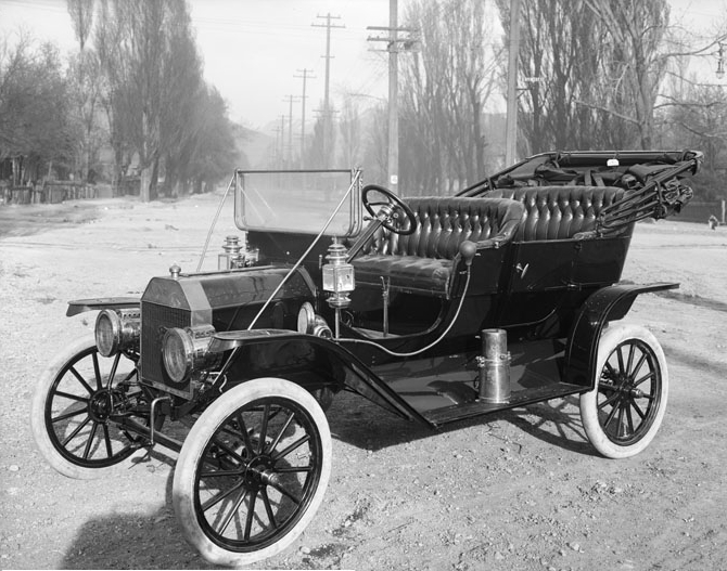
- Ford introduced the moving assembly line in 1908.
- The new model T was mass produced instead of hand assembled.
- The new production method drove the cost of model T down, making it affordable to more consumers.
- Model T sold millons over the next 20 years.
- Ford Motor Company transformed from a small startup to the leading automobile company.
5.4.4. Game On

- William Durant incorporated General Motors.
- There were about 45 different car companies in the US, most of them selling a handful of cars.
- General Motors was the opposite of Ford.
- It produced a wide variety of cars for a wide variety of consumer needs.
- In the first 2 years, General Motors cobbled together 30 companies, 11 of which where automakers.
5.4.5. The Market Leader
- Model T's production innovations made Ford the leading car company from about 1910 to 1925.
- The reluctance of Ford to keep introducing innovations and the absence of flexibility changed the situation.
- In 1925, GM surpassed Ford in total revenue and kept ahead until 1986.
- Eventually in 1927, Ford shutdown for 6 months to update its production lines for Model A.
- GM also surpassed Ford in total sales during this period.
5.5. Leader-follower Competition in Quantities
- The Stackelberg model of oligopoly describes a market structure with two or more firms such that
- the market does not suffer from any other market failure (imperfect information, externalities, etc),
- no other firms can enter the market,
- firms sell a homogeneous product,
- firms try to maximize their profits,
- consumers are price takers, firms choose the quantities that they produce, the leader chooses first, and the follower(s) choose afterward, and
- consumers try to maximize their utility.
5.5.1. Residual Demand
- The leader chooses the quantity it produces first.
- Thus, the follower does not face the entire market demand but only the demand remaining after the leader's choice.
- The difference between the market demand and the aggregated supplied quantities of all competitive firms is a firm's residual demand.
5.5.2. The Follower's Problem
- We solve the problem with backward induction.
- The follower claims the residual demand.
- For any given quantity \(q_{1}\) produced by the leader, the follower's problem is
\[\max_{q_{2}} \left\{ p(q_{1} + q_{2})q_{2} - c_{2}(q_{2}) \right\}.\]
- Interior optimal solutions require
\[p'(q_{1} + q_{2})q_{2} + p(q_{1} + q_{2}) = c_{2}'(q_{2}).\]
- From this condition, we obtain (solving for \(q_{2}\)) the best response of the follower, say
\[q_{2} = b_{2}(q_{1}).\]
5.5.3. The Leader's Problem
- The leader anticipates the best response of the follower and solves
\[\max_{q_{1}} \left\{ p(q_{1} + b_{2}(q_{1}))q_{1} - c_{1}(q_{1}) \right\}.\]
- Its optimality condition is given by
\[p'(q_{1} + b_{2}(q_{1})) \left(1 + b_{2}'(q_{1})\right) q_{1} + p(q_{1} + b_{2}(q_{1})) = c_{1}'(q_{1}).\]
5.5.4. An Analytic Example
Suppose that the demand and cost functions are given by
\begin{align*} p(q) &= p_{0} + p_{1} q, \\ c_{1}(q_{1}) &= c q_{1}, \\ c_{2}(q_{2}) &= c q_{2}. \end{align*}
5.5.5. The Follower's Problem
- The follower's necessary condition becomes
\[p_{1}q_{2} + p_{0} + p_{1}(q_{1} + q_{2}) = c.\]
- Then, the best response of the follower is
\[b_{2}(q_{1}) = \frac{c - p_{0} - p_{1}q_{1}}{2 p_{1}}.\]
5.5.6. The Leader's Problem
- The leader solves
\[\max_{q_{1}} \left\{ p\left(q_{1} + \frac{c - p_{0} - p_{1}q_{1}}{2 p_{1}}\right)q_{1} - c(q_{1}) \right\}.\]
- Its optimality condition is given by
\[\frac{p_{1}}{2}q_{1} + p_{0} + \frac{c - p_{0}}{2} + \frac{p_{1}}{2}q_{1} = c.\]
- Therefore, the leader produces
\[q_{1}^{\ast} = \frac{c - p_{0}}{2 p_{1}}.\]
5.5.7. Market Quantity and Price
- Given the leader's quantity, the follower produces
\[q_{2}^{\ast} = b_{2}(q_{1}^{\ast}) = \frac{c - p_{0}}{2 p_{1}} - \frac{1}{2}\frac{c - p_{0}}{2 p_{1}} = \frac{c - p_{0}}{4 p_{1}}.\]
- The market quantity is
\[q^{\ast} = q_{1}^{\ast} + q_{2}^{\ast} = 3\frac{c - p_{0}}{4 p_{1}}.\]
- The market price is
\[p(q^{\ast}) = p_{0} + p_{1} q^{\ast} = \frac{p_{0} + 3 c}{4}.\]
5.5.8. Profits
- The follower makes profit
\[\pi_{2} = \left(p(q^{\ast}) - c\right) q_{2}^{\ast} = - \frac{\left(p_{0} - c\right)^{2}}{16p_{1}}.\]
- The leader's profit is
\[\pi_{1} = \left(p(q^{\ast}) - c\right) q_{1}^{\ast} = - \frac{\left(p_{0} - c\right)^{2}}{8p_{1}}.\]
5.5.9. First Move Advantage
- The firms' profits in the Cournot model with symmetric costs are
\[\pi_{c} = - \frac{\left(p_{0} - c\right)^{2}}{9p_{1}}.\]
- Compared to the firms' profits in the Cournot model, we have
\[\pi_{1} > \pi_{c} > \pi_{2}.\]
- The leader makes more profit compared to Cournot competition, while the follower makes less profit.
- However, aggregate profits in the market are less compared to Cournot, i.e.,
\[\pi_{1} + \pi_{2} < 2 \pi_{c}.\]
5.6. Leader-Follower Competition in Prices
- Consider a variation of the Stackelberg game in which firms are price setters.
- This is the sequential version of the Bertrand model.
- There are two firms \((i, j \in \{1,2\})\) with marginal cost equal to \(c\).
- Firm \(1\) is the leader (moves first), and firm \(2\) is the follower (moves second).
The demand for firm \(i\) is
\begin{align*} d_{i}(p_{i}, p_{j}) = \left\{\begin{aligned} &10 - \frac{1}{2}p_{i} & p_{i} < p_{j} \\ &5 - \frac{1}{4}p_{i} & p_{i}=p_{j} \\ &0 & p_{i} > p_{j} \end{aligned}\right.. \end{align*}- The firm with the lowest price gets all the demand.
- If prices are equal, demand is equally split.
5.6.1. Non Equilibrium Prices
- Suppose that firm \(1\) sets a price \(p_{1}\) that is greater than the marginal cost of firm \(2\) (i.e., \(c\)).
- Firm \(2\) can undercut by a small amount and grab all the market. For instance, set price \(p_{2} = \frac{c + p_{1}}{2}\).
- Thus, firm \(1\) can only set a price equal to firm \(2\)'s marginal cost.
5.6.2. Equilibrium
- The only possible equilibrium is both firms to set a price equal to the (common) marginal cost.
- Firms do not have any incentive to deviate.
- Setting lower prices leads to losses.
- Setting higher prices leads to zero profits.
- The order with which firms move does not affect the market outcome.
5.7. A Game of Market Entry
- Consider a market with one firm already operating and a potential entrant.
- The entrant decides whether to enter the market.
- The incumbent decides whether to follow aggressive or complying competition behavior.
5.7.1. Entry Deterrence with Credible Threat
5.8. Quantity Competition with Costly Entry
- We extend the Cournot duopoly model by allowing firms to choose whether they enter the market.
- Firms enter the market when they can make profits.
- Firms incur a fixed cost \(\bar c\) upon entry.
5.8.1. Market and Dynamics
- There is an infinite number of potential entrants.
- The market's inverse demand is
\[p(q) = p_{0} + p_{1}q \quad(p_{0}>0,\ p_{1}<0).\]
- All firms have costs
\[c(q) = c_{1}q \quad(c_{1}>0).\]
- The firms that enter the market choose their quantities at the second date simultaneously.
- At the first date, the entrants decide how many of them enter the market.
5.8.2. Unregulated Entry and Exit
- When \(n\) firms enter the market, each firm makes profit
\[\pi_{i}(n) = -\frac{(c_{1} - p_{0})^{2}}{(n + 1)^{2} p_{1}} - \bar c.\]
- In equilibrium
\[\pi_{i}(n^{e}) = 0 \iff n^{e} = \frac{p_{0} - c_{1}}{\sqrt{- \bar c p_{1}}} - 1.\]
5.8.3. The Social Welfare
5.8.4. The First Best Solution
- Aggregate profit is maximized when
\[p(n q(n))\left(q(n) + n q'(n)\right) - c(q(n)) - n c'(q(n))q'(n) = \bar c .\]
- This implies that
\[n^{*} = \sqrt[3]{-\frac{(p_{0} - c_{1})^{2}}{p_{1} \bar c}} - 1 .\]
- Comparing with the unregulated entry equilibrium, we have
\[ n^{*} < n^{e} .\]
- With quantity competition, unregulated entry results in excessive entry of firms.
5.9. Current Field Developments
- Market dynamics and entry constitute important components of competition policy.
- Mergers and acquisitions are dynamic phenomena modifying the number of firms in the market and their market power.
- Merger cases are central from both an economic and competition law perspective.
- In the US and EU, antitrust laws aim to reduce or avoid excessive market concentration.
- Dynamic market models are commonly used to assess mergers and their impact on market power in court cases.
5.10. Concise Summary
- The sequence with which firms act in a market can influence market power.
- If firms compete in quantities, then the leader has a first move advantage.
- If firms compete in prices, then the sequence of moves is irrelevant.
- Competition forces do not concern only firms who already entered in a market.
- Incumbent firms strategically interact with potential competitors looking to enter the market.
- Free entry is a characteristic of market competition that can reduce firms' profits and result to low prices.
- On some occasions (e.g. entry costs), excessive entry can result to economic inefficiencies.
5.11. Further Reading
- Watson (2008, chaps. 15, 16)
- Belleflamme and Peitz (2010, secs. 4.1, 4.2.1-3)
- Varian (2010, secs. 28.2, 29.8)
5.12. Mathematical Details
5.12.1. Leader-follower duopoly with quantity competition and asymmetric costs
Firms choose their strategies sequentially. The leader chooses first, and the follower chooses afterward. Both firms choose their supplied quantities. The oligopoly of sequential quantity competition is known as the Stackelberg model.
- The follower's problem
The leader anticipates the follower's actions and takes them into account when optimizing. We use this idea to solve the problem using backward induction. The follower's problem is \[\max_{q_{2}} \left\{ p(q_{1} + q_{2}) q_{2} - c_{2}(q_{2}) \right\}.\]
- The follower's best response
Using a variational argument, we get \[p'(q_{1} + q_{2}) q_{2} + p(q_{1} + q_{2}) = c_{2}'(q_{2}).\] This condition determines the best response of the follower when the leader strategy is given by \(q_{2}\). Say that this relation is given by \(b_{2}(q_{1})\).
- The leader's problem
The leader solves \[\max_{q_{1}} \left\{ p(q_{1} + b_{2}(q_{1})) q_{1} - c_{1}(q_{1}) \right\}.\] Its optimality condition is given by \[p'(q_{1} + b_{2}(q_{1})) (1 + b_{2}'(q_{1})) q_{1} + p(q_{1} + b_{2}(q_{1})) = c_{1}'(q_{1}).\]
- An affine demand, linear costs example
For inverse demand and costs given by
\begin{align*} p(q) &= p_{0} + p_{1} q \\ c_{1}(q) &= \kappa_{1} q \\ c_{2}(q) &= \kappa_{2} q, \end{align*}the best response function of the follower becomes \[b_{2}(q_{1}) = \frac{\kappa_{2} - p_{0} - p_{1} q_{1}}{2 p_{1}}.\] The leader optimally chooses \[q_{1} = \frac{2\kappa_{1} - \kappa_{2} - p_{0}}{2 p_{1}}.\] Thus, the follower subsequently chooses \[q_{2} = \frac{3\kappa_{2} - 2\kappa_{1} - p_{0}}{4 p_{1}}.\]
- Market prices and quantities
The total quantity in the market is
\begin{align*} q &= q_{1} + q_{2} \\ &= \frac{2\kappa_{1} - \kappa_{2} - p_{0}}{2 p_{1}} + \frac{3\kappa_{2} - 2\kappa_{1} - p_{0}}{4 p_{1}} \\ &= \frac{2 \kappa_{1} + \kappa_{2} - 3 p_{0}}{4 p_{1}}. \end{align*}The price can be calculated by the inverse demand function as \[p(q) = p_{0} + p_{1} \frac{2 \kappa_{1} + \kappa_{2} - 3 p_{0}}{4 p_{1}} = \frac{2 \kappa_{1} + \kappa_{2} + p_{0}}{4}.\]
- Profits
The leader has profit \[\pi_{1} = \left( \frac{2 \kappa_{1} + \kappa_{2} + p_{0}}{4} - \kappa_{1} \right) q_{1} = - \frac{\left(2 \kappa_{1} - \kappa_{2} - p_{0}\right)^{2}}{8 p_{1}},\] and the follower has profit \[\pi_{2} = \left( \frac{2 \kappa_{1} + \kappa_{2} + p_{0}}{4} - \kappa_{2} \right) q_{2} = - \frac{\left(3 \kappa_{2} - 2\kappa_{1} - p_{0}\right)^{2}}{8 p_{1}}.\]
5.12.2. A Stackelberg Competition Example
Suppose that there are two firms in the market. Firm \(1\) is the leader, and firm \(2\) is the follower.Let the cost function of both firms be \[c_{i}(q_{i}) = 4 q_{i}.\] Let market inverse demand be \[p(q_{1} + q_{2}) = 28 - 2 \left(q_{1} + q_{2}\right).\]
The follower's problem is \[\max_{q_{2}} \left\{ \left(28 - 2 \left(q_{1} + q_{2}\right)\right) q_{2} - 4 q_{2} \right\},\] and the necessary condition gives \[28 - 2 q_{1} - 4 q_{2} = 4.\] This condition determines the best response of the follower when the leader produces \(q_{1}\). \[q_{2} = \frac{24 - 2q_{1}}{4}.\] Then, the leader solves \[\max_{q_{1}} \left\{ \left(28 - 2 \left(q_{1} + \frac{24 - 2q_{1}}{4}\right) \right) q_{1} - 4 q_{1} \right\}.\] Its optimality condition is given by \[12 - 2 q_{1} = 0.\]
Solving for \(q_{1}\), we find that the leader is optimally producing \(q_{1} = 6\). We can substitute \(q_{1} = 6\) back to the follower's best response to get the follower's quantity \[q_{2} = \frac{24 - 2q_{1}}{4} = 3.\] The market quantity is the sum of the firms' quantities \[q = q_{1} + q_{2} = 9.\] The market price can then be calculated by the inverse demand function \[p = p(q) = 10.\]
Finally, the leader has profit \[\pi_{1} = P q_{1} - 4 q_{1} = 36,\] and the follower's profit is \[\pi_{2} = P q_{2} - 4 q_{2} = 18.\] The leader has a first move advantage and its profit is greater than the follower's.
5.13. Exercises
5.13.1. Group A
Consider an endogenous timing game in which firms simultaneously choose whether to play \(Early\) or to play \(Late\) . If both firms make the same choice, then they compete as in the Bertrand competition. If the firms make different choices, then they compete as in the Stackelberg model (sequential competition in quantities), where the leader is the firm that chose \(Early\) and the follower is the firm that chose \(Late\). Suppose that firms have cost functions to \(c(q)=q\), and market demand is given by \(p(q) = 5 - q\).
- Calculate the profits of the firms under the different means of competition.
- Draw the extensive form of the game.
- Calculate all the Nash Equilibria.
- If the firms compete simultaneously using prices, they set \(p_{1} = p_{2} = 1\) and make zero profits. If they compete sequentially using quantities, the follower makes profit \[\pi_{f} = \frac{(5-1)^{2}}{16} = 1,\] and the leader makes profit \[\pi_{l} = \frac{(5-1)^{2}}{8} = 2.\]
- The extensive form of the game is
- There are two pure strategy Nash equilibria, namely \[\left\{\left\{Early, Late\right\}, \left\{Late, Early\right\}\right\},\] and a mixed strategy equilibrium in which each firm chooses \(Early\) with probability \(p=\frac{2}{3}\).
Suppose that there are two firms in a market with an affine inverse demand function \(p(q) = p_{0} + p_{1}q\), where \(p_{0}>0\) and \(p_{1}<0\). The firms have constant marginal costs equal to \(c\) and no fixed production cost. Show that the leader in a leader-follower duopoly with quantity competition has a first move advantage. Specifically, show that the leader's profit is always greater than the profit it would attain in a market with simultaneous quantity competition.
In the leader-follower problem, the leader makes profit
\begin{align*} \pi_{l} = - \frac{(c_{1} - p_{0})^2}{8 p_{1}} . \end{align*}In the simultaneous move game, each firm makes profit
\begin{align*} \pi_{s} = -\frac{(c_{1} - p_{0})^{2}}{9 p_{1}}. \end{align*}One can calculate the ratio of the profits
\begin{align*} \frac{\pi_{l}}{\pi_{s}} = \frac{(c_{1} - p_{0})^2}{8 p_{1}} \frac{9 p_{1}}{(c_{1} - p_{0})^{2}} = \frac{9}{8} > 1, \end{align*}which implies that \(\pi_{l}>\pi_{s}\).
Consider a market with inverse market demand function \(p(q) = 100 - 2q\). The total cost function for any firm in the market is given by c(q) = 4q. Suppose that the market consists of two firms that compete by choosing their supplied quantities. Firm 1 is the market leader, while firm 2 is the follower. Calculate the firms' optimally supplied quantities, total market output, and market price.
The follower takes prices as given and solves
\begin{align*} \max_{q_{2}} \left\{ p(q_{1} + q_{2}) q_{2} - c(q_{2}) \right\}, \end{align*}which determines the best response of the follower as
\begin{align*} b_{2}(q_{1}) = \frac{48 - q_{1}}{2}. \end{align*}Then, the leader solves
\begin{align*} \max_{q_{1}} \left\{ p\left(q_{1} + \frac{48 - q_{1}}{2}\right) q_{1} - 4 q_{1} \right\} = \max_{q_{1}} \left\{ \left(48 - q_{1}\right) q_{1} \right\}, \end{align*}which determines the optimal supplied quantity of the leader as \(q_{1} = 24\). Substituting into the best response of the follower results in \(q_{2} = 12\). The market quantity is \(q_{s} = q_{1} + q_{2} = 36\), and the market price is
\begin{align*} p(q_{s}) = 100 - 72 = 28. \end{align*}
5.13.2. Group B
Consider the quantity competition with costly entry game. Suppose that firms face market demand \(p(q) = p_{0} + p_{1}q\), have symmetric production costs \(c(q)=c_{1}q\), and entry costs \(\bar c\), where \(p_{0}, c_{1} > 0\) and \(p_{1}<0\). The social welfare as a function of the number of firms is given by \[W(n) = \int_{0}^{n} p(s q(s)) \left(q(s) + sq'(s)\right) \mathrm{d} s - n c(q(n)) - n \bar c .\] Calculate the Pareto optimal number of entrants in the market.
By Fermat's theorem, the welfare is maximized when \(W'(n) = 0\). Using the fundamental theorem of calculus, we get \[p(n q(n))\left(q(n) + n q'(n)\right) - c(q(n)) - n c'(q(n))q'(n) = \bar c.\] The optimal quantity produced by each firm when \(n\) firms enter the market is \[q(n) = -\frac{p_{0} - c_{1}}{(n + 1) p_{1}},\] hence, one calculates \[\frac{q'(n)}{q(n)} = \frac{1}{n + 1}.\] We will use the last expression to simplify the first order condition. Rearranging the necessary condition and using the linearity of costs gives
\begin{align*} \bar c &= p(n q(n))\left(q(n) + n q'(n)\right) - c(q(n)) - n c'(q(n))q'(n) \\ &= p(n q(n))q(n) - c(q(n)) + n \left(p(n q(n)) - c'(q(n))\right)q'(n) \\ &= \pi(n) + n \left(p(n q(n))q(n) - c(q(n))\right) \frac{q'(n)}{q(n)} \\ &= \pi(n) \left(1 + n \frac{q'(n)}{q(n)}\right) \\ &= \pi(n) \left(1 - n \frac{1}{n + 1}\right) \\ &= \pi(n) \left(\frac{1}{n + 1}\right). \end{align*}The profit of each firm when \(n\) firms enter the market is \[\pi(n) = -\frac{(p_{0} - c_{1})^{2}}{(n + 1)^{2} p_{1}},\] so, we get
\begin{align*} \bar c &= -\frac{(p_{0} - c_{1})^{2}}{(n + 1)^{3} p_{1}}. \end{align*}Therefore, the socially optimal number of firms is given by
\begin{align*} n &= \sqrt[3]{-\frac{(p_{0} - c_{1})^{2}}{p_{1} \bar c}} - 1. \end{align*}
6. Collusion and Market Power
6.1. Context
- Markets with intense competition tend to reduce the competing firms' market power. Firms could form cartels to control the market and extract a greater share of the economic surplus if left unregulated. For this reason, collusion and cartel formation are illegal practices in most market economies today.
- However, legally binding contracts are not necessary for firms to coordinate. Firms can use dynamic strategies to collude tacitly.
- What kind of strategies can lead to tacit collusion?
- What is the role of the means of competition in tacit collusion?
- How can competition authorities measure market power?
6.2. Course Structure Overview
6.3. Lecture Structure and Learning Objectives
Structure
- Our Customers are Our Enemies (Case Study)
- Tacit Collusion
- Trigger Strategies with Quantity Competition
- Trigger Strategies with Price Competition
- Market Power
- Current Field Developments
Learning Objectives
- Illustrate that in dynamic settings, credible promises and threats can be used to induce tacit collusion.
- Illustrate that tacit collusion is achievable both when firms compete in quantities and prices
- Describe tacit collusion under price competition.
- Describe tacit collusion under quantity competition.
- Explain how market power can be statistically measured and estimated.
6.4. Our Customers are Our Enemies
- Lysine is an amino acid that speeds the development of lean muscle tissue in humans and animals.
- It is essential for humans, but we cannot synthesize it.
- It has to be obtained from the diet.
6.4.1. The Lysine Industry
- At the end of the 1980s, the world lysine industry consisted of three significant sellers:
- Ajinomoto,
- Kyowa, and
- Sewon.
- The three largest consumption regions were Japan, Europe, and North America.
- Most production took place in Japan, but it was based on imports of US dextrose.
- Ajinomoto had the largest share of the world market.
6.4.2. The ADM Entry
- In February 1991, Archer Daniel Midland Co. (ADM) entered the market and built by far the world's largest lysine plant in the US.
- ADM hired biochemist Mark Whitacre, Ph.D., as head of the new division.
- ADM's plant was three times the size of Ajinomoto's largest plant.
- ADM gave Ajinomoto and Kyowa executives an unrestricted tour to show its production capacity.
- Companies engaged in a price war.
- Three months before ADM's entry, the average US lysine price was \($1.22\) per pound.
- After an 18-month price war, the US price averaged \($0.68\) per pound.
- ADM's share of the US market reached \(80\%\).
6.4.3. The Lysine Association
- After the price war, ADM was willing to soften competition.
- In 1992, Mark Whitacre and his boss Terrance Wilson met with top Ajinomoto and Kyowa managers.
- Wilson proposed forming a world lysine association that would regularly meet.
- The new association would collect and distribute market information.
- Wilson also suggested that the new association could provide a convenient cover for illegal price-fixing discussions! (Connor 2001)
- After a year, the lysine association was founded, met quarterly, and performed the two functions that Wilson proposed.
6.4.4. Price Fixing
 Connor (2000)
- There were \(25\) price fixing meetings in total.
- The first one took place in the Nikko Hotel in Mexico on June 23, 1992.
- The average Lysine price immediately jumped by more than \(12\%\).
- Consensus was not always easy to reach. The companies distrusted each other!
- There was a breakdown of the cartel during the spring and summer of 1993, and the lysine price plummeted.
- The crisis was resolved at a meeting in Irvine, California in October 1993 between ADM's and Ajinomoto Executives. But…
- This meeting and many others were caught on video by the FBI.
6.4.5. Frenemies
WILSON: The only thing we need to talk here because we are gonna get manipulated by these God damn buyers, they're sh, they can be smarter than us if we let them be smarter.
MIMOTO: (Laughs).
WILSON: Okay?
MIMOTO: (ui).
WILSON: They are not your friend. They are not my friend. And we gotta have 'em. Thank God we gotta have 'em, but they are not my friends. You're my friend. I wanna be closer to you than I am to any customer. 'Cause you can make us, I can make money, I can't make money. At least in this kind of a market. And all I wanna is ta tell you again is let's-let's put the prices on the board.
Co-conspirator explains how end-of-year compensation scheme eliminates incentives to cheat on cartel
6.4.6. The Whistle-blower
- In 1992, Mark Whitacre became an FBI whistle-blower. He is the highest-level corporate executive to ever have done so.
- Whitacre's wife pressured him into becoming a whistle-blower. She threatened to inform the FBI herself if Whitacre wouldn't do it.
- Whitacre informed the FBI that he and other ADM executives performed illegal price-fixing operations.
- Over the next three years, Whitacre collected information and recorded conversations with ADM executives and competitors.
- The ADM settlement involved the greatest US federal charges at the time.
- Whitacre was convicted for embezzling and money laundering, which he performed while cooperating with the FBI in the price fixing case.
6.4.7. What can we Learn?
- Why did ADM initially engage in a price war?
- Why did it initiate the price fixing discussions afterward?
- Why was there so much distrust among companies?
6.5. Tacit Collusion
- When there is a future, firms can use reputation and/or threats to coordinate.
- Coordination increases their profits.
- Explicit contracts are not needed.
- Trigger strategies can induce coordination.
- Trigger strategies work both when firms compete in quantities and prices.
6.6. Tacit Collusion in Quantity Competition
- When coordinating, firms produce at the monopolistic level and split the market.
- Alternatively, firms play their static Cournot strategies.
- On every date, there are two potential game states.
- Either both firms have always cooperated in the past.
- Or, at least one of them deviated.
- The trigger strategy is to produce the monopolistic quantity at state 1 and the Cournot quantity at state 2.
6.6.1. The Problem
- Suppose that both firms discount future profits by \(\delta \in (0,1)\).
- Firms aim to maximize the series of discounted flow profits, i.e.,
\[V_{i} = \max_{(q_{i,t})_{t}} \left\{ \sum_{t=0}^{\infty} \delta^{t} \pi_{i,t}(q_{1,t}, q_{2,t}) \right\}.\]
6.6.2. Non Coordinating Equilibrium
- There are many equilibria in the game.
- The non coordinating equilibrium is one in which the stage game Nash equilibrium is played at every date.
- All firms use the oligopolistic quantity competition production levels at every date, which leads to flow profits
\[\pi_{i,t} = - \frac{(c_{1}-p_{0})^{2}}{9 p_{1}} \quad\quad (i=1,2\quad t\ge 0).\]
- Each firm's expected future series of profits is
\[V_{i} = - \frac{1}{1-\delta}\frac{(c_{1}-p_{0})^{2}}{9 p_{1}} \quad\quad (i=1,2\quad t\ge 0).\]
6.6.3. Coordinating Equilibrium with Trigger Strategies
- Another equilibrium can be obtained when firms play the trigger strategies.
- Firms produce half the monopolistic quantity and split the monopolistic profits, i.e.,
\[\pi_{i,t} = - \frac{1}{2}\frac{(c_{1}-p_{0})^{2}}{4 p_{1}} \quad\quad (i=1,2\quad t\ge 0).\]
- If firms coordinate with these profits as flow utilities, they get
\[V_{m, i} = - \frac{1}{1-\delta}\frac{(c_{1}-p_{0})^{2}}{8 p_{1}} \quad\quad (i=1,2\quad t\ge 0).\]
6.6.4. Deviating from Coordination
- Is there any incentive to deviate?
- Suppose that firm 1 deviates at the current date.
- The best response to firm 2's choice of monopolistic profits is
\[q_{1,0} = \frac{3}{8}\frac{c_{1}-p_{0}}{p_{1}}.\]
- Then, firm 1's profit at the current date is
\[\pi_{1,t} = - \frac{9}{64}\frac{(c_{1}-p_{0})^{2}}{p_{1}}.\]
- On future dates, the firms revert to the non coordinating quantities because they use trigger strategies.
- The total discounted profit of the deviating firm is
\[V_{d,1} = - \frac{9}{64}\frac{(c_{1}-p_{0})^{2}}{p_{1}} - \frac{\delta}{1 - \delta} \frac{(c_{1}-p_{0})^{2}}{9 p_{1}}.\]
6.6.5. Can Coordination be Supported?
- The coordination outcome is sustainable if the deviation profit is less than the coordination profit, namely if
- This is equivalent to \(\delta > \frac{9}{17}\).
- As long as firms value future profits enough, there is room for cooperation.
6.7. Tacit Collusion in Price Competition
- When coordinating, firms produce at the monopolistic level and split the market.
- Alternatively, firms play their static Bertrand strategies.
- On every date, there are two potential states.
- Either both firms have always cooperated in the past.
- Or, at least one of them deviated.
- The trigger strategy is to use the monopoly price at state 1 and the Bertrand price at state 2.
6.7.1. The Problem
- Suppose again that both discount future profits by \(\delta \in (0,1)\).
- Firms aim to maximize the series of discounted flow profits, i.e.,
\[V_{i} = \max_{(p_{i,t})_{t}} \left\{ \sum_{t=0}^{\infty} \delta^{t} \pi_{i,t}(p_{1,t}, p_{2,t}) \right\}.\]
6.7.2. Non Coordinating Equilibrium
- Firms price at marginal cost when non coordinating.
- They make zero profits at each date.
- Therefore, \(V_{i}=0\).
6.7.3. Coordinating Equilibrium with Trigger Strategies
- As in the case of quantity competition, if firms produce half the monopolistic quantity and split the monopolistic profits, they get
\[\pi_{i,t} = - \frac{1}{2}\frac{(c_{1}-p_{0})^{2}}{4 p_{1}} \quad\quad (i=1,2\quad t\ge 0).\]
- If firms coordinate, then
\[V_{m, i} = - \frac{1}{1-\delta}\frac{(c_{1}-p_{0})^{2}}{8 p_{1}} \quad\quad (i=1,2\quad t\ge 0).\]
6.7.4. Deviating from Coordination
- Suppose that firm 1 deviates at the current date.
- The best response to firm 2's choice of monopolistic pricing is to slightly undercut the market price by \(\varepsilon\)
- Then, firm 1 takes all the market and makes almost the monopolistic profit
- For simplicity, drop \(\varepsilon\), so that
\[\pi_{1,t} = - \frac{(c_{1}-p_{0})^{2}}{4 p_{1}}.\]
- On future dates, the firms have zero profits because they use trigger strategies.
- The total discounted profit of the deviating firm is
\[V_{d,1} = - \frac{(c_{1}-p_{0})^{2}}{4 p_{1}}.\]
6.7.5. Can Coordination be Supported?
The coordination outcome is sustainable if the deviation profit is less than the coordination profit, namely if
\begin{align*} V_{1,d} &= - \frac{(c_{1}-p_{0})^{2}}{4 p_{1}} \\ &< - \frac{1}{1 - \delta} \frac{(c_{1}-p_{0})^{2}}{8 p_{1}} = V_{1,m}. \end{align*}- This is equivalent to \(\delta > \frac{1}{2}\).
- As long as firms value future profits enough, there is room for cooperation.
- Why is the lower bound \(\delta\) in quantity competition greater than in price competition?
6.8. Market Power
- In legal cases of competition law, market power is a central element based on which decisions are drawn.
- Market power refers to the ability of the firm to raise prices above marginal cost (the perfectly competitive price level).
- Marginal cost is not always observable, so it is not always easy to assess market power.
6.8.1. The Lerner Index
- The Lerner index (usually denoted \(L\)) is defined by the markup, i.e., the difference between price and marginal cost, as a percentage of the price.
\[L = \frac{p-c'}{p}\]
- Prices are observed, but marginal costs are typically not, and firms are not always eager to reveal this information.
6.8.2. Concentration Index
- A concentration index is a statistic that measures the degree of concentration of the market. A market is concentrated when only a few firms have a large share of the market.
- The concentration ratio is the sum of the market shares of a subset of firms in the market. For example, with \(n\) firms in the market, \(\alpha_{i} = q_{i} / Q\) denoting the share of firm \(i\), and a \(M\) denoting a subset firms, the M-concentration ratio is given by
\[I_{M} = \sum_{i\in M} \alpha_{i}.\]
- If \(I_{m}\) is close to one, it means that most of the market is controlled by the \(m\) firms included in the calculation.
- If \(m\) is small, this suggests that the market is concentrated.
6.8.3. Herfindahl Index
- The Herfindahl Index is a statistic that measures the degree of concentration of the market by considering the full distribution of market shares. It is defined as the sum of squares (\(\mathcal{L}^2\) norm) of market shares of all active firms in the market.
- For \(n\) firms in the market, with \(\alpha_{i} = q_{i} / Q\) denoting the share of firm \(i\), the Herfindahl index is
\[I_{H} = \sum_{i=1}^{n} \alpha_{i}^{2}.\]
- The closer is the value of \(I_{H}\) to one, the more concentrated the market is.
6.8.4. Estimating Market Power
- Suppose that we know the inverse market demand \(p(q;x)\), where \(q\) is the market quantity and \(x\) is a vector of other exogenous characteristics affecting demand.
- One approach to estimating market power is to start from the equation
\[MR(\lambda) = p + \lambda p'(q;x) q\]
- If \(\lambda=0\), then \(MR(\lambda) = p\), i.e., the market is perfectly competitive.
- If \(\lambda=1\), then the market is a monopoly, i.e.,
\[MR(\lambda) = p + p'(q;x) q.\]
- If \(\lambda=1/n\), then the market is represented by a symmetric \(n\text{-firm}\) Cournot model, i.e.,
\[MR(\lambda) = p + \frac{1}{n}p'(q;x) q.\]
6.8.5. Equilibrium
- Suppose that \(c'(q;w)\) is the marginal cost function, where \(w\) is a vector of exogenous characteristics affecting cost.
- In equilibrium, for all firms in the market, it holds
\[p = c'(q;w) - \lambda p'(q;x) q.\]
- From this expression, we can obtain estimates of \(\lambda\).
6.9. Current Field Developments
- Recent work further investigates methods for estimating market power.
- There is a plethora of methods for estimating market power (Perloff, Karp, and Golan 2007).
- Recent antitrust cases in the EU are those against Google for Goggle Shipping and Google AdSense.
- Google has been fined with over \(8\) billion Euro for these cases.
- In 2020, a case has been filed against Facebook in the US for suppressing competition from social media rivals.
6.10. Concise Summary
- Firms can employ trigger strategies to induce collusion in the market.
- Explicit use of contracts is not required.
- Collusion can be sustained both under quantity and price competition.
- Quantity competition requires firms to value future profits more than price competition.
- Market power can be measured by statistics such as the Herfindahl index.
- Market power can be estimated using a variation of the first order condition of the Cournot model.
6.11. Further Reading
- Watson (2008, chaps. 22, 23)
- Belleflamme and Peitz (2010, secs. 2.3, 3.5, 14.2.1)
- Varian (2010, secs. 28.10, 28.11)
6.12. Mathematical Details
6.12.1. Repeated simultaneous quantity competition with two firms
When there is a future, firms can use reputation and/or threats to coordinate without explicitly cooperating. This gives them the ability to increase their profits. A simple threat that can induce coordination is the trigger strategy.
- The trigger strategy
The goal of the trigger strategy is that the firms produce at the monopolistic level and split the market. If any firm deviates from this strategy, the other firm reverts to producing the oligopolistic quantity for all future dates.
- The problem
Suppose that there are two firms in the market. Both discount future profits by \(\delta \in (0,1)\). Let demand be affine and costs linear. Firms aim to maximize the series of flow profits, i.e., \[V_{i} = \max_{(q_{i,t})_{t}} \left\{ \sum_{t=0}^{\infty} \delta_{t} \pi_{i,t}(q_{1,t}, q_{2,t}) \right\}.\]
- Non coordinating equilibrium
There are many equilibria in the game. A simple equilibrium is one that the stage game Nash equilibrium is played are every date. All firms use the oligopolistic quantity competition production levels at every date, which leads to flow profits \[\pi_{i,t} = - \frac{(c_{1}-p_{0})^{2}}{9 p_{1}} \quad\quad (i=1,2\quad t\ge 0).\] Therefore, each firm's expected future series of profits is \[V_{i} = - \frac{1}{1-\delta}\frac{(c_{1}-p_{0})^{2}}{9 p_{1}} \quad\quad (i=1,2\quad t\ge 0).\]
- Coordinating equilibrium with trigger strategies
Another equilibrium can be obtained when firms play the trigger strategies. Firms produce half the monopolistic quantity and split the monopolistic profits \[\pi_{i,t} = - \frac{1}{2}\frac{(c_{1}-p_{0})^{2}}{4 p_{1}} \quad\quad (i=1,2\quad t\ge 0).\] If firms coordinate with these profits as flow utilities, they get \[V_{m, i} = - \frac{1}{1-\delta}\frac{(c_{1}-p_{0})^{2}}{8 p_{1}} \quad\quad (i=1,2\quad t\ge 0).\]
Is there any incentive to deviate? Suppose that Firm 1 deviates at the current date. The best response to Firm 2's choice of monopolistic profits is \[q_{1,0} = \frac{3}{8}\frac{c_{1}-p_{0}}{p_{1}}.\] Then, firm 1's profit at the current date is \[\pi_{1,t} = - \frac{9}{64}\frac{(c_{1}-p_{0})^{2}}{p_{1}}.\] On future dates, the firms revert to the non coordinating quantities because they use trigger strategies. Therefore, the total discounted profit of the deviating firm is \[V_{d,1} = - \frac{9}{64}\frac{(c_{1}-p_{0})^{2}}{p_{1}} - \frac{\delta}{1 - \delta} \frac{(c_{1}-p_{0})^{2}}{9 p_{1}}.\]
The coordination outcome is sustainable if the deviation profit is less than the coordination profit, namely if
\begin{align*} V_{1,d} &= - \frac{9}{64}\frac{(c_{1}-p_{0})^{2}}{p_{1}} - \frac{\delta}{1 - \delta} \frac{(c_{1}-p_{0})^{2}}{9 p_{1}} \\ &< - \frac{1}{1 - \delta} \frac{(c_{1}-p_{0})^{2}}{8 p_{1}} = V_{1,m}, \end{align*}which is equivalent to \(\delta > \frac{9}{17}\). Thus, as long as firms value future profits enough, there is room for cooperation.
6.13. Exercises
6.13.1. Group A
Consider two firms competing in quantities for an infinite number of dates. The discount factor is \(\delta \in (0, 1)\).The market's inverse demand is \(p(q)=220-q\), and both firms have a marginal cost equal to \(10\)
- Find the equilibrium under non cooperation (Cournot competition) at each date. Calculate the quantity that a monopolist would produce at each date. Calculate the profits in both cases and compare them.
- Write down the trigger strategies of the two firms that can lead to tacit collusion.
- What is the most profitable deviation from the trigger strategy at the initial date? What is the profit of the deviation at this date? How does the profit compare with the coordination profit of the trigger strategy?
- For which values of \(\delta\) is collusion sustainable?
In the stage game, each firm maximizes \[\max_{q_{i}} (220 - q_{i} - q_{j} - 10 ) q_{i},\] which implies that \(q_{i} = q_{j} = q_{c} = 70\). When firms do not cooperate, they choose to produce these quantities at all dates. In this case, the market price is \[p(2q_{c}) = 220 - 140 = 80,\] and each firm makes profit \[\pi_{c} = (80 - 10 ) 70 = 4900.\]
The monopolist would instead maximize \[\max_{q} (220 - q - 10 ) q,\] which gives \(q_{m} = 105\). The market price is then \[p(q_{m}) = 220 - 105 = 115,\] and the monopolist makes profit \[\pi_{m} = (115 - 10) 105 = 11025.\]
The trigger strategy that can lead to collusion is for each firm \(i\) to produce according to the rule
\begin{align*} q_{i,t} = \left\{ \begin{aligned} \frac{q_{m}}{2} & \quad\quad q_{j,s}=\frac{q_{m}}{2} \text{ for all } s < t \\ q_{c} & \quad\quad \text{ otherwise } \end{aligned}\right. . \end{align*}- Given that firm \(j\) plays the trigger strategy, firm \(i\) maximizes \[\max_{q_{i}} \left(220 - q_{i} - \frac{105}{2} - 10\right) q_{i},\] which implies that the best firm \(i\) can do, if it deviates from the trigger strategy, is to produce \(q_{d} = \frac{315}{4}\). The profit of firm \(i\) is then \[\pi_{d} = \frac{99225}{16},\] which is greater than \(pi_{m}/2\). Thus, the firm can make greater flow profit at the initial date if it deviates from coordination.
- This practice, however, does not make the firm overall better off. Only short-sighted firms prefer this scenario. Firms that value future profits prefer coordination. Specifically, coordination can be sustained if and only if \[\frac{1}{1-\delta} \frac{\pi_{m}}{2} \ge \pi_{d} + \frac{\delta}{1 -\delta}\pi_{c}\] or equivalently \[\delta \ge \frac{\frac{\pi_{m}}{2} - \pi_{d}}{\pi_{c}- \pi_{d}} = \frac{\frac{11025}{2} - \frac{99225}{16}}{4900 - \frac{99225}{16}} = \frac{11025}{20825} = \frac{9}{17}.\]
Consider two firms competing in prices for a potentially infinite number of dates. The two firms have marginal costs equal to \(c\). If the two firms set the same price, they split the market so that firm \(1\) gets a share \(\mu\) and firm \(2\) gets a share \(1-\mu\). The firms do not discount future profits, but there is a probability \(p > 0\) that the market closes down after each date. The firms use trigger strategies to coordinate and split the monopolistic profit.
- Find the equilibrium if \(p=1\).
- Suppose that \(\mu = \frac{1}{2}\). Find the values of \(p<1\) for which collusion is sustainable. How do you interpret the result?
- Find the values of \(p<1\) for which collusion is sustainable for any value of \(\mu\in(0,1)\). What is the equilibrium relationship between \(p\) and \(\mu\)? How do you interpret the result?
- If \(p=1\), the firms compete only for one date, and the game reduces to Bertrand competition. The firms set \(p_{1}=p_{2}=c\).
- The most profitable deviation of each firm at the initial date is to slightly undercut the monopoly price by \(\varepsilon\). By doing so, the firm can take all the market demand and achieve almost the monopolistic profit. For simplicity, assume that the deviating firm earns exactly the monopolistic profit. Then, the deviation is not profitable if and only if \[\frac{1}{p}\frac{\pi_{m}}{2} \ge \pi_{m} \iff p \le \frac{1}{2}.\] Collusion is sustainable if the probability that the market closes down is small and the firms have the potential to benefit from future profits.
- With arguments analogous to the \(\mu=\frac{1}{2}\) case, the condition for firm \(1\) is \[\frac{1}{p}\mu \pi_{m} \ge \pi_{m} \iff p \le \mu,\] and for firm \(2\) is \[\frac{1}{p}(1-\mu) \pi_{m} \ge \pi_{m} \iff p \le 1-\mu.\] Therefore, collusion is sustainable if and only if \[p \le \min\{\mu, 1-\mu\}.\] If \(\mu < \frac{1}{2}\), the equilibrium condition becomes less stringent when \(\mu\) increases. In contrast, the equilibrium condition becomes more stringent when \(\mu\) increases for \(\mu>\frac{1}{2}\). The most lenient equilibrium condition is obtained for \(\mu=\frac{1}{2}\). The further is \(\mu\) from \(\frac{1}{2}\), the less are the flow profits that one of the two firms makes and, as a result, coordination based on future benefits becomes less profitable.
6.13.2. Group B
Consider two firms competing in quantities for an infinite number of dates. The discount factor is \(\delta \in (0, 1)\).The market's inverse demand is \(p(q)=p_{0}+p_{1}q\) and both firms have marginal cost equal to \(c\), where \(p_{0}>c>0\) and \(p_{1}<0\). Suppose that firms use the following tit-for-tat strategy. If the other firm has produced half the monopolistic quantity last date, then produce half the monopolistic quantity at this date. Otherwise, produce the Cournot quantity.
- Find the equilibrium under non cooperation (Cournot competition) at each date. Calculate the profits of the firms.
- Find the total discounted profits if each firm produces half the monopolistic quantity at each date.
- Find the most profitable deviation of firm \(i\) at the initial date. Calculate the profit of the deviating firm at the initial date.
- Suppose that at the second date, the deviating firm reverts to producing half the monopolistic quantity. Calculate the profit it makes at this date.
- For which values of \(\delta\) is collusion sustainable?
- As in the grim trigger strategy case, if the firms do not coordinate, they produce \[q_{c} = \frac{c - p_{0}}{3 p_{1}},\] make flow profits \[\pi_{c} = -\frac{(p_{0} - c)^{2}}{9 p_{1}},\] and total discounted profits \[V_{c} = -\frac{1}{1-\delta}\frac{(p_{0} - c)^{2}}{9 p_{1}}.\]
- In this case, each firm produces \[\frac{q_{m}}{2} = \frac{c - p_{0}}{4 p_{1}},\] makes flow profit \[\frac{\pi_{m}}{2} = -\frac{(p_{0} - c)^{2}}{8 p_{1}},\] and total discounted profit \[V_{m} = -\frac{1}{1-\delta}\frac{(p_{0} - c)^{2}}{8 p_{1}}.\]
- The most profitable deviation of firm \(i\) is calculated by solving \[\max_{q_{i}} \left(p_{0} + p_{1} \left(q_{i} + \frac{q_{m}}{2}\right) - c\right) q_{i},\] which leads to \[q_{1} = \frac{3}{8}\frac{c-p_{0}}{p_{1}},\] and flow profit \[\pi_{1} = -\frac{9}{64}\frac{(c-p_{0})^{2}}{p_{1}}.\]
Firm \(i\) is producing half the monopolistic quantity, and firm \(j\) is producing the Cournot quantity, punishing the initial date deviation. Thus, firm \(i\) makes profit
\begin{align*} \pi_{2} &= \left(p_{0} + p_{1} \left(\frac{q_{m}}{2} + q_{c}\right) - c\right) \frac{q_{m}}{2} \\ &= -\frac{5}{48}\frac{(c-p_{0})^{2}}{p_{1}}. \end{align*}There are two cases we should consider. The deviating firm may revert back to producing half the monopolistic quantity after the deviation, or it can resort to producing the Cournot quantity. In the first case, the payoff is \[V_{r} = \pi_{1} + \delta \pi_{2} + \delta^{2} V_{m},\] while in the second case, it is \[V_{n} = \pi_{1} + \delta V_{c}.\] The second case is excluded if and only if
\begin{align*} V_{r} \ge V_{n} &\iff \pi_{2} + \delta V_{m} \ge V_{c} \\ &\iff -\frac{5}{48}\frac{(c-p_{0})^{2}}{p_{1}} - \frac{\delta}{1-\delta} \frac{1}{8}\frac{(c-p_{0})^{2}}{p_{1}} \ge - \frac{1}{1-\delta} \frac{1}{9}\frac{(c-p_{0})^{2}}{p_{1}} \\ &\iff \delta \ge \frac{1}{3}. \end{align*}Moreover, for collusion to be sustainable, we need
\begin{align*} V_{m} \ge V_{r} &\iff V_{m} \ge \pi_{1} + \delta \pi_{2} + \delta^{2} V_{m} \\ &\iff -\frac{1 - \delta^{2}}{1-\delta} \frac{1}{8} \frac{(c-p_{0})^{2}}{p_{1}} \ge -\frac{9}{64}\frac{(c-p_{0})^{2}}{p_{1}} - \delta \frac{5}{48}\frac{(c-p_{0})^{2}}{p_{1}} \\ &\iff (1 + \delta) \frac{1}{8} \ge \frac{9}{64} + \delta \frac{5}{48} \\ &\iff \delta \ge \frac{3}{4}. \end{align*}